Scoring metrics in the Splunk Machine Learning Toolkit
In the Splunk Machine Learning Toolkit (MLTK), the score command runs statistical tests to validate model outcomes. You can use the score command for robust model validation and statistical tests in any use case.
MLTK uses the following classes of the score command, each with their own sets of methods:
- Classification
- Clustering
- Pairwise distances scoring
- Regression scoring
- Statistical functions (statsfunctions)
- Statistical testing (statstest)
The Splunk Machine Learning Toolkit also enables the examination of how well your model might generalize on unseen data by using folds of the training set. This method is known as k-fold scoring. The kfold command does not use the score command, but operates as a type of scoring.
Score commands cannot be customized within the Splunk Machine Learning Toolkit.
Classification
You can use classification scoring metrics to evaluate the predictive power of a classification learning algorithm.
Classification scoring in the Splunk Machine Learning Toolkit includes the following methods:
- Accuracy
- Confusion matrix
- F1-score
- Precision
- Precision-Recall-F1-Support
- Recall
- ROC-AUC-score
- ROC-curve
Overview
The most common use of classification scoring is to evaluate how well a classification model performs on the test set. The inputs to the classification scoring methods are actual and predicted fields, corresponding to ground-truth-labels and predicted-labels, respectively. The syntax also supports the comparison of multiple fields, allowing for multi-field comparisons. This is useful for evaluating which classification model is best suited for your data.
Classification scoring methods only work on categorical data such as integers and string-types, but not on floats. These methods are used to evaluate the output of classification algorithms, such as logistic regression. You may see an error message if you attempt to use the comparison scoring method on numeric float-type data.
Preprocessing
All classification scoring methods follow the same preprocessing steps:
- Search commands are pulled into memory.
- The data is prepared:
- All rows containing NAN values are removed prior to computing the score.
- You may receive an error if any categorical fields are found.
Parameters
- The
pos_labelparameter must be an element of all actual or ground truth data. - An error will display if the a valid value for
pos_labelis not found in an actual field. - Use the
pos_labelparameter to specify the positive class whenaverage=binary. - The
pos_labelparameter is ignored if the average is not binary. - The
averageparameter includes several options including None, Binary, Micro, Macro and Weighted.
Parameter option for average
|
Use cases |
|---|---|
| None | Returns the scoring metric for each unique class in the union of actual_field + predicted_field.
|
| Binary | Reports results for the class specified by the pos_label parameter. This parameter only works for binary data and will display an error if applied to a multiclass problem.
|
| Micro | Calculates metrics globally by counting the total true-positives, false-negatives, and false-positives. |
| Macro | Calculates metrics for each label and finds their unweighted mean. Does not take label imbalance into account. |
| Weighted | Calculates metrics for each label and finds their average weighted by support as in the number of true instances for each label. This alters the Macro to account for label imbalance and can result in an F-score that is not between Precision and Recall. |
Syntax
As with all scoring methods, classification methods support pairwise comparisons between two sets of fields or arrays. The general syntax is as follows:
.. | score <scoring-method-name> array_a against array_b [options]
- The
againstparameter separates the ground-truth fields (on the left) from the predicted fields."~"is equivalent. array_arepresents the ground-truth fields, and is specified by fieldsactual_field_1 ... actual_field_narray_brepresents the predicted fields, and is specified by fieldspredicted_field_1 ... bpredicted_field_n
SPL syntax
.. | score <scoring-method-name> <actual_field_1> ... <actual_field_n> against <predicted_field_1> ... <predicted_field_n> [options]
Syntax constraints
Classification scoring supports the wildcard (*) character in cases of 1-to-n only.
Examples
The following example shows the loaded data split into training (<=70 partitions) and testing (>70 partitions) sets. Classification scoring is used, and the model saved as a knowledge object.
The training set is selected, and the model is applied to get predictions on unseen data, perform scoring, and analysis of the results.
The following syntax example is training multiple models on the same field.
| inputlookup iris.csv

| sample partitions=100 seed=1234
| search partition_number <= 70

| fit LogisticRegression species from * into LR_model
| fit RandomForestClassifier species from * into RF_model
| fit GaussianNB species from * into GNB_model
| fit DecisionTreeClassifier species from * into DT_model
The following syntax example is evaluating the ground truth field against multiple predictions.
| inputlookup iris.csv

| sample partitions=100 seed=1234
| search partition_number > 70

| apply LR_model as LR_species
| apply RF_model as RF_species
| apply GNB_model as GNB_species
| apply DT_model as DT_species

| score precision_recall_fscore_support species ~ LR_species RF_species GNB_species DT_species average=weighted
The following visualization shows the evaluation of the ground truth field against multiple predictions.
Accuracy scoring
Use accuracy scoring to get the prediction accuracy between actual-labels and predicted-labels.
Accuracy scoring implements sklearn.metrics.accuracy_score. Learn more here: http://scikit-learn.org/stable/modules/generated/sklearn.metrics.accuracy_score.html
Further reading: https://en.wikipedia.org/wiki/Accuracy_and_precision
Parameters
- The
normalizeparameter default is True. - The
normalizeparameter dictates whether to return the raw count of correctly classified samples (normalize=False) or the fraction of correctly classified samples (normalize=True). - When the
pos_labelparameteraverage=binaryand the combined cardinality of the actual or predicted field is <= 2, the report results forclass=pos_labelonly.
Syntax
...|score accuracy_score <actual_field_1> ... <actual_field_n> against <predicted_field_1> ... <predicted_field_n> normalize=<True|False>
Syntax constraints
- Accuracy scoring supports 1-to-1, n-to-n, and 1-to-n comparison syntaxes.
- Accuracy scoring supports the wildcard (*) character in cases of 1-to-n only.
Example
You manually specify fields because a predicted field exists in the data. In particular, manually specify fields for second call to the fit command and onwards.
| inputlookup track_day.csv

| sample partitions=100 seed=1234
| search partition_number <= 70

| fit LogisticRegression vehicleType from batteryVoltage engineCoolantTemperature engineSpeed into LR_model
| fit DecisionTreeClassifier vehicleType from batteryVoltage engineCoolantTemperature engineSpeed into DT_model
After training a classifier to predict vehicle type, you can analyze your test set accuracy.
| inputlookup track_day.csv

| sample partitions=100 seed=1234
| search partition_number > 70

| apply LR_model as LR_prediction
| apply DT_model as DT_prediction
| score accuracy_score vehicleType against LR_prediction DT_prediction
Example output
Confusion matrix
Use the confusion matrix to evaluate the accuracy between actual-labels and predicted-labels.
Implements sklearn.metrics.confusion_matrix. Learn more here: http://scikit-learn.org/stable/modules/generated/sklearn.metrics.confusion_matrix.html
Further reading: https://en.wikipedia.org/wiki/Confusion_matrix
Parameters
The confusion matrix takes no parameters.
Syntax
score confusion_matrix <actual_field> against <predicted_field>
Syntax constraints
- The
ground-truth-labelsmap along the vertical event axis, and thepredicted-labelsmap along the horizontal field-axis. - Works only for 1-1 comparisons, because the output of
confusion_matrixis already 2d. - Confusion matrix scoring does not support the wildcard (*) character.
Although order is not preserved in the output fields and events, the correspondence of fields and events is preserved.
Example
The following example uses a confusion matrix to test actual vehicle type against predicted vehicle type.
| inputlookup track_day.csv

| sample partitions=100 seed=1234
| search partition_number > 70

| apply DT_model as DT_prediction

| score confusion_matrix vehicleType against DT_prediction
Example output
The following visualization of the confusion matrix shows which classes were most and least successfully predicted, as well as what they were mistaken for.
F1-score
Compute the F1-score between true-labels and predicted-labels.
Implements sklearn.metrics.f1_score. Learn more here: http://scikit-learn.org/stable/modules/generated/sklearn.metrics.f1_score.html
Further reading: https://en.wikipedia.org/wiki/F1_score
Parameters
- The
pos_labelparameter default is 1. - When the
pos_labelparameteraverage=binaryand the combined cardinality of the actual or predicted field is <= 2, the report results forclass=pos_labelonly. - The
averageparameter default is binary.
Syntax
|score f1_score <actual_field_1> ... <actual_field_n> against <predicted_field_1> ... <predicted_field_n> average=<binary(default) | micro | macro | weighted> pos_label=<str | int>
Syntax constraints
- F1-score supports 1-to-1, n-to-n, and 1-to-n comparison syntaxes.
- F1-score supports the wildcard (*) character in cases of 1-to-n only.
Example
The following example tests the prediction of vehicle type using F1-score.
| inputlookup track_day.csv

| sample partitions=100 seed=1234
| search partition_number <= 70

| fit LogisticRegression vehicleType from batteryVoltage engineCoolantTemperature engineSpeed into LR_model
| fit DecisionTreeClassifier vehicleType from batteryVoltage engineCoolantTemperature engineSpeed into DT_model
After training a classifier to predict vehicle type, you can evaluate your model's precision on the training set for each vehicle type.
| inputlookup track_day.csv

| sample partitions=100 seed=1234
| search partition_number > 70

| apply LR_model as LR_prediction
| apply DT_model as DT_prediction

| score f1_score vehicleType against LR_prediction DT_prediction average=micro
Example output
The following visualization shows the F1-score model on a test set for each vehicle type with LogisticRegression results on the left and DecisionTree results on the right. The visualization also shows the average across all vehicle types.
Precision
Compute the Precision score between actual-labels and predicted-labels. Assess the ability of the classifier to not label a positive sample as a negative sample.
Implements sklearn.metrics.precision_score. Learn more here:http://scikit-learn.org/stable/modules/generated/sklearn.metrics.precision_score.html
Further reading: https://en.wikipedia.org/wiki/Accuracy_and_precision
Parameters
- The
pos_labelparameter default is 1. - When the
pos_labelparameteraverage=binaryand the combined cardinality of the actual or predicted field is <= 2, the report results forclass=pos_labelonly. - The
averageparameter default is binary.
Syntax
...|score precision_score <actual_field_1> ... <actual_field_n> against <predicted_field_1> ... <predicted_field_n> average=<binary(default)|micro|macro|weighted> pos_label=<str|int>
Syntax constraints
- Precision scoring supports 1-to-1, n-to-n and 1-to-n. comparison syntaxes.
- Precision scoring supports the wildcard (*) character in cases of 1-to-n only.
Example
The following example tests the prediction of vehicle type using precision scoring.
| inputlookup track_day.csv

| sample partitions=100 seed=1234
| search partition_number <= 70

| fit LogisticRegression vehicleType from batteryVoltage engineCoolantTemperature engineSpeed into LR_model
| fit DecisionTreeClassifier vehicleType from batteryVoltage engineCoolantTemperature engineSpeed into DT_model
After training a classifier to predict vehicle type, you can evaluate the model's precision on the training set for each vehicle type.
| inputlookup track_day.csv

| sample partitions=100 seed=1234
| search partition_number > 70

| apply LR_model as LR_prediction
| apply DT_model as DT_prediction

| score precision_score vehicleType against LR_prediction DT_prediction average=None
Example output
The following visualization shows the precision model on a test set for each vehicle type with LogisticRegression results on the left and DecisionTree results on the right. A warning shows that rows containing NAN values and have been removed.
Precision-Recall-F1-Support
Compute the Precision, Recall, F1-score, and support between actual-fields and predicted-fields.
Implements sklearn.metrics.precision_recall_fscore_support. Learn more here: http://scikit-learn.org/stable/modules/generated/sklearn.metrics.precision_recall_fscore_support.html
Parameters
- The
pos_labelparameter default is 1. - When the
pos_labelparameteraverage=binaryand the combined cardinality of the actual or predicted field is <= 2, the report results forclass=pos_labelonly. - The
averageparameter default is None. - The
betaparameter default is 1.0. - The
betaparameter shows the strength of recall versus precision inf-score.
Syntax
score precision_recall_fscore_support <actual_field_1> ... <actual_field_n> against <predicted_field_1> ... <predicted_field_n> pos_label=<str> average=<str> beta=<float>
Syntax constraints
You can refer to the following table to distinguish your results when average=None and when average=Not None.
| Average | Result |
|---|---|
| Not None | Works for all syntax constraints including 1-to-1 and 1-to-n. |
| None | Only works for 1-1 comparisons because the output of precision_recall_fscore_support is already 2d. Support scoring is only defined when average=None because averaged values are not generated for support.
|
Precision-Recall-F1-Support supports the wildcard (*) character in cases of 1-to-n only.
Example
The following example tests the prediction of vehicle type using Precision-Recall-F1-Support scoring.
| inputlookup track_day.csv

| sample partitions=100 seed=1234
| search partition_number <= 70

| fit LogisticRegression vehicleType from batteryVoltage engineCoolantTemperature engineSpeed into LR_model
| fit DecisionTreeClassifier vehicleType from batteryVoltage engineCoolantTemperature engineSpeed into DT_model
After training a classifier to predict vehicle type, you can evaluate your model's precision on the training set for each vehicle type.
| inputlookup track_day.csv

| sample partitions=100 seed=1234
| search partition_number > 70

| apply LR_model as LR_prediction
| apply DT_model as DT_prediction

| score precision_recall_fscore_support vehicleType against LR_prediction DT_prediction average=weighted
Example output
The following visualization shows the precision, recall, and f_beta scores for the prediction of vehicle type, under a weighted averaging scheme.
Recall
Compute the Recall score between actual-labels and predicted-labels.
Implements sklearn.metrics.recall_score. Learn more here: http://scikit-learn.org/stable/modules/generated/sklearn.metrics.recall_score.html
Further reading: https://en.wikipedia.org/wiki/Precision_and_recall
Parameters
- The
pos_labelparameter default is 1. - When the
pos_labelparameteraverage=binaryand the combined cardinality of the actual or predicted field is <= 2, the report results forclass=pos_labelonly. - The
averageparameter default is binary.
Syntax
|score recall_score <actual_field_1> ... <actual_field_n> against <predicted_field_1> ... <predicted_field_n> average=<binary(default) | micro | macro | weighted> pos_label=<str | int>
Syntax constraints
- Recall supports 1-to-1, n-to-n, and 1-to-n comparison syntaxes.
- Recall partially supports the wildcard (*) character in cases of 1-to-n only.
Example
The following example tests the prediction of vehicle type using recall scoring.
| inputlookup track_day.csv

| sample partitions=100 seed=1234
| search partition_number <= 70

| fit LogisticRegression vehicleType from batteryVoltage engineCoolantTemperature engineSpeed into LR_model
| fit DecisionTreeClassifier vehicleType from batteryVoltage engineCoolantTemperature engineSpeed into DT_model
After training a classifier to predict vehicle type you can evaluate your model's precision on the training set for each vehicle type.
| inputlookup track_day.csv

| sample partitions=100 seed=1234
| search partition_number > 70

| apply LR_model as LR_prediction
| apply DT_model as DT_prediction

| score recall_score vehicleType against LR_prediction DT_prediction average=weighted
Example output
The following visualization shows the recall model on a test set with LogisticRegression results on the left and DecisionTree results on the right. The visualization shows the average across all vehicle types where the average is weighted by the support.
ROC-AUC-score
Compute the ROC-AUC curve between actual-labels and predicted-scores.
Implements sklearn.metrics.roc_auc_score. Learn more here: http://scikit-learn.org/stable/modules/generated/sklearn.metrics.roc_auc_score.html
Further reading: https://en.wikipedia.org/wiki/Receiver_operating_characteristic
Parameters
- Although
sklearn.metrics.roc_auc_scoresupports anaverageparameter, this parameter is disabled as MLTK does not support thelabel-indicatorformat. - The
pos_labelparameter default is 1. - You can use the
pos_labellabel when data is multi class but you want to apply binary scoring methods. Thepos_labellabel allows multiclass data to cast to binary by specifying the class identified aspos_labelas the positive class, and all other classes as negative. For the original multiclass data ofa, b, c, a, ewhenpos_label=athe resulting binary data is1, 0, 0, 1, 0. - When the predicted field contains target scores, that field can either be probability estimates of the positive class, confidence values, or a non-thresholded measure of decisions.
Requirements
- ROC-AUC-score only applies to binary data. To support multi-class problems, binarize the data using the
pos_labelparameter. - The predicted field must be numeric. The numeric data must be float or integer type, corresponding to probability estimates of the positive class, confidence values, or a non-thresholded measure of decisions as returned by the
decision_functionparameter on some classifiers. - If the predicted field does not meet the numeric criteria, an error message will display.
| If | Then |
|---|---|
| Binary data is given | The data must be true binary such as {0,1} or {-1,1}. |
| Binary is not data such as multiclass | The pos_label parameter must be specified and contained in the ground_truth field.
|
| Binary is not true binary | The pos_label parameter must be specified and contained in the ground_truth field.
|
If the pos_label parameter is not in the ground_truth field, an error message will display.
If the ground truth data is multiclass and the pos_label parameter is properly specified, you may see an error message.
Syntax
score roc_auc_score <actual_field_1> ... <actual_field_n> against <predicted_field_1> ... <predicted_field_n> pos_label=<str | int>
Syntax constraints
- ROC-AUC-score supports 1-to-1, n-to-n, and 1-to-n comparison syntaxes.
- ROC-AUC-score does not support the wildcard (*) character.
Example
The following example shows how you can obtain the area under the ROC curve for predicting the vehicle type of 2013 Audi RS5.
| inputlookup track_day.csv

| sample partitions=100 seed=1234
| search partition_number <= 70

| fit LogisticRegression vehicleType from * probabilities=True into LR_model
| inputlookup track_day.csv

| sample partitions=100 seed=1234
| search partition_number > 70

| score roc_auc_score vehicleType against "probability(vehicleType=2013 Audi RS5)" pos_label="2013 Audi RS5"
Example output
The following visualization shows the results of the ROC-AUC scoring on a test set.
ROC-curve
Compute the ROC-curve between actual-fields and predicted-fields.
Implements sklearn.metrics.roc_curve. Learn more here: http://scikit-learn.org/stable/modules/generated/sklearn.metrics.roc_curve.html
Further reading: https://en.wikipedia.org/wiki/Receiver_operating_characteristic
Parameters
- The
pos_labelparameter default is 1. - You can use the
pos_labellabel when data is multiclass but you want to apply binary scoring methods. Thepos_labellabel allows multiclass data to cast to binary by specifying the class identified aspos_labelas the positive class, and all other classes as negative. The original multiclass data ofa, b, c, a, ewhenpos_label=aresults in the binary data of1, 0, 0, 1, 0. - The
drop_intermediateparameter default is True. Whether to drop sub optimal thresholds which would not appear on a plotted ROC-curve. This is useful when creating lighter ROC curves.
Requirements
- ROC-curve only applies to binary data. To support multiclass problems, convert the data into binary with the
pos_labelparameter. - The predicted field must be numeric. The numeric data must be float or integer type, corresponding to probability estimates of the positive class, confidence values, or non-thresholded measure of decisions.
- If the predicted field does not meet the numeric criteria, an error message will display.
| If | Then |
|---|---|
| Binary data is given | It must be true-binary such as {0,1} or {-1,1}. |
| Binary is not data such as multiclass | The pos_label parameter must be specified and contained in the ground_truth field.
|
| Binary is not true binary | The pos_label parameter must be specified and contained in the ground_truth field.
|
If the pos_label parameter is not in the ground_truth field, an error message displays.
If the ground truth data is multiclass and the pos_label is properly specified, you are warned of the conversion.
Syntax
score roc_curve <actual_field> against <predicted_field> pos_label=<str|int> drop_intermediate=<True|False>
Syntax constraints
- ROC-curve scoring only works for 1-1 comparisons.
- ROC-curve scoring does not support the wildcard (*) character.
Example
The following example tests the probability of churn using ROC-curve scoring.
| inputlookup churn.csv

| sample partitions=100 seed=1234
| search partition_number <= 70

| fit LogisticRegression Churn? from * probabilities=True into LR_model
| inputlookup churn.csv

| sample partitions=100 seed=1234
| search partition_number > 70

| apply LR_model probabilities=True
| score roc_curve Churn? against "probability(Churn?=True.)" pos_label='True.'
Example output
The following visualization shows how the true positive rate (tpr) varies with the false positive rate (fpr), along with the corresponding probability thresholds.
Clustering scoring
You can use clustering scoring to evaluate the predicted value of a clustering model. The inputs to the clustering scoring methods are arrays of data specified by an ordered sequence of fields.
Clustering scoring in the Splunk Machine Learning Toolkit includes the following methods:
Overview
Clustering scoring methods can operate on two arrays. The label and features fields are specified by the ordered sequence of the fields <label_field> and feature_field_1 feature_field_2 ... feature_field_n respectively.
You can use the against clause to separate the arrays where label_field against feature_field_1 feature_field_2 ... feature_field_n correspond to label (ground truth or predicted labels) against features (features used by clustering algorithm), respectively.
Clustering scoring methods will only work on numerical data, and are expected to be used to evaluate the output of clustering models such as KMeans and Spectral Clustering. Attempting to score on categorical data will display an error.
Neither parameters that take a list or array as input or metrics that calculate the distance between categorical arrays are supported.
Preprocessing
Clustering scoring methods perform the following preprocessing steps:
- Search commands are pulled into memory.
- The data is prepared:
- All rows containing NAN values are removed prior to computing the score.
- The
labelfield is converted to categorical. - An error message displays if any categorical fields are found in the feature fields.
Parameters
- The
metricparameter default is euclidean. - Supported
metricvalues include: cityblock, cosine, euclidean, l1, l2, manhattan, braycurtus, canberra, chebyshev, correlation, hamming, matching, minkowski, and sqeuclidean. - The wildcard (*) character is disabled for clustering scoring methods.
- The number of fields in the
label_arrayparameter is limited to one and it must be categorical.
Silhouette score
You can use the silhouette score to calculate the prediction accuracy between label_array and feature_array.
Implements sklearn.metrics.silhouette_score. Learn more here: http://scikit-learn.org/stable/modules/generated/sklearn.metrics.silhouette_score.html
Further reading: https://en.wikipedia.org/wiki/Silhouette_(clustering)
Parameters
Silhouette score supports clustering scoring parameters.
Syntax
...|score silhouette_score <label_field> against <feature_field_1> ... <feature_field_n> metric=<euclidean(default) | cityblock | cosine | l1 | l2 | manhattan | braycurtis | canberra | chebyshev | correlation | hamming | matching | minkowski | sqeuclidean>
Syntax constraints
Silhouette score supports the following syntax constraints:
label_fieldparameter must have only single field.feature_fieldsparameter can have single or multiple fields.- Silhouette score supports the wildcard (*) character in cases of 1-to-n only.
Example
The following example uses silhouette scoring to calculate species prediction on a test data set.
| inputlookup iris.csv
| fit StandardScaler petal_length petal_width sepal_length sepal_width as scaled
| fit KMeans scaled_* k=3 as KMeans_predicted_species
| score silhouette_score KMeans_predicted_species against scaled_petal_length scaled_petal_width scaled_sepal_length scaled_sepal_width
Example output
The following visualization shows the results of silhouette scoring on the iris dataset.
Pairwise distances scoring
You can use pairwise distances scoring to calculate the distances between different fields.
Pairwise distances scoring in the Splunk Machine Learning Toolkit includes the following methods:
Overview
The inputs to the pairwise distances scoring methods are array(s) of data specified by an ordered sequence of fields. The arrays for pairwise distances scoring methods are a_array and b_array.
Pairwise distances scoring methods support pairwise comparisons between two sets of fields or arrays such as a_field_1 a_field_2 ... a_field_n and b_field_1, b_field_2, b_field_m respectively. The general syntax is as follows:
..| score <scoring-method-name> a_field_1 a_field_2 ... a_field_n against b_field_1 b_field_2 ... b_field_m [options]
The against clause separates arrays. The "~" symbol is equivalent.
In general, statistical methods are commutative such that a_field against b_field is equivalent to b_field against a_field. The arrays a_array and b_array are specified by a sequence of fields: a_field_1 ... a_field_n and b_field_1 ... b_field_m.
Pairwise distances scoring methods only work on numerical data. Attempting to score on categorical data will display an error.
Preprocessing
All pairwise distance scoring methods follow the same preprocessing steps:
- Search commands are pulled into memory.
- The data is prepared:
- All rows containing NAN values are removed prior to computing the score.
- An error message displays if any categorical fields are found in both arrays.
Parameters
- The
metricparameter default = euclidean. - Supported
metricvalues include: cityblock, cosine, euclidean, l1, l2, manhattan, braycurtis, canberra, chebyshev, correlation, hamming, matching, minkowski, sqeuclidean, Kolmogorov-Smirnov (2 samples), and Wasserstein distance. - The
outputparameter default = matrix. - Pairwise distances scoring supports the wildcard (*) character.
- Supported output values are matrix and list.
Using metric values of Kolmogorov-Smirnov (2 samples) or Wasserstein distance requires running version 1.4 of the Python for Scientific Computing add-on.
Some parameters have not been supported:
- Parameters that take a list or array as input.
- Metrics that calculate the distance between categorical arrays.
Pairwise distances score
Calculate the pairwise distances score between a_array and b_array.
Implements sklearn.metrics.pairwise.pairwise_distances. Learn more here: http://scikit-learn.org/0.19/modules/generated/sklearn.metrics.pairwise.pairwise_distances.html
Parameters
Pairwise distances score score supports pairwise distances scoring parameters.
- The metric parameter default =
euclidean. - Supported metric values include: cityblock, cosine, euclidean, l1, l2, manhattan, braycurtis, canberra, chebyshev, correlation, hamming, matching, minkowski, sqeuclidean Kolmogorov-Smirnov (2 samples), and Wasserstein distance.
- The output parameter default =
matrix. - Supported output values are matrix and list.
- In cases of event-vs-event distances Pairwise distances support only field-vs-field (column-wise) distances. If you need to calculate the distances between events you can transpose the matrix first and then use the
pairwise_distancesscore command. - Pairwise distances scoring supports the wildcard (*) character.
Using metric values of Kolmogorov-Smirnov (2 samples) or Wasserstein distance requires running version 1.4 of the Python for Scientific Computing add-on.
Syntax
...|score pairwise_distances <a_field_1> ... <a_field_n> against <b_field_1> ... <b_field_m> metric= <euclidean(default) | cityblock | cosine | l1 | l2 | manhattan | braycurtis | canberra | chebyshev | correlation | hamming | matching | minkowski | sqeuclidean | ks_2samp | wasserstein_distance> output=<matrix(default) | list>
Syntax constraints
a_fieldcan have single or multiple fields with numbers that may be equal to each other, or differ from each other.b_fieldcan have single or multiple fields with numbers that may be equal to each other, or differ from each other.
Examples
The following example uses pairwise distances scoring on a test set.
| inputlookup iris.csv
| score pairwise_distances petal_length petal_width AGAINST sepal_length sepal_width
The following visualization shows pairwise distance scoring on a test set.
The following example uses the output=list parameter.
| inputlookup iris.csv
| score pairwise_distances petal_length petal_width AGAINST sepal_length sepal_width output=list
The following visualization shows pairwise distance scoring on a test set including the output=list parameter.
The following example uses event-vs-event distances on a test set.
| inputlookup iris.csv
| table petal* sepal*
| transpose 0
The following visualization shows event-vs-event distances on a test set.
The following example uses the output=list parameter on a test set. .
| inputlookup iris.csv
| table petal* sepal*
| transpose 0
| score pairwise_distances "row 1" "row 2" AGAINST "row 3" "row 4"  output=list | fields *_fields pairwise*
The following visualization shows the output=list parameter on a test set.
Regression scoring
Use regression scoring metrics to evaluate the predictive power of a regression learning algorithm. The most common use of regression scoring is to evaluate how well a regression model performs on the test set.
Regression scoring in the Splunk Machine Learning Toolkit includes the following methods:
The inputs to the regression scoring methods are arrays of data specified by an ordered sequence of fields.
Regression scoring methods can operate on two arrays. The actual and predicted fields are specified by an ordered sequence of fields actual_field_1 .. actual_field_n and predicted_field_1 ... predicted_field_n, respectively.
You can use the against clause to separate the arrays where actual_field_1 ... actual_field_n against predicted_field_1 ... predicted_field_n correspond to to actual (ground truth target values) against predicted (predicted target values), respectively.
These scoring methods only work on numerical data, and are used to evaluate the output of regression algorithms such as Gradient Boosting Regression and Linear Regression.
Attempting to score on categorical data, or having no numerical fields in any of the arrays displays an error.
Preprocessing
Regression scoring methods follow the same preprocessing steps:
- Search commands are pulled into memory.
- The data is prepared:
- All rows containing NAN values are removed prior to computing the score.
- An error message displays if any categorical fields are found in the feature fields.
Parameters
- The
multioutputparameter default israw_values. - The
raw_valuesparameter returns a full set of regressions scores or errors between each field infields_aandfield_brespectively. - The wildcard (*) character is supported in cases of 1-to-n only.
- The number of fields in
actual_fieldsandpredtcted_fieldsmust be either equal to each other or one of them must have only one field. - If one of the arrays has a single field and the other array has multiple fields, the
multioutputparameter is set toraw_values. - If one of the arrays has a single field and the other array has multiple fields, the regression score is calculated between each field of the array which has multiple fields and the one field of the array that has a single field.
- If the
multioutputparameter was set to a different value by the user beforehand, an error displays.
Parameters that take a list or array as input are not supported.
Explained variance score
You can use explained variance score to calculate the explained variance regression score between predicted and actual fields.
Implements sklearn.metrics.explained_variance_score. Learn more here: http://scikit-learn.org/stable/modules/generated/sklearn.metrics.explained_variance_score.html#sklearn.metrics.explained_variance_score
Further reading: https://en.wikipedia.org/wiki/Explained_variation
Parameters:
- The
multioutputparameter default israw_values. - The
variance_weightedparameter is the scores of all outputs averages with the weights of each individual output's variance. - To see each explained variance score compared to the actual score, set the multioutput parameter to
raw_values.
Syntax
...|score explained_variance_score <actual_field_1> ... <actual_field_n> against <predicted_field_1> ... <predicted_field_n> multioutput=<raw_values(default) | uniform_average | variance_weighted>
Syntax constraints
- Explained variance score supports 1-to-1, n-to-n, and 1-to-n comparison syntaxes.
- Explained variance score supports the wildcard (*) character in 1-to-n cases.
Explained variance score is not symmetric.
Example
The following example shows manually specified fields in particular for the second call to the fit command and onwards because a predicted field exists in the data.
| inputlookup server_power.csv
| fit LinearRegression ac_power from total-cpu-utilization total-disk-accesses total-disk-utilization as ac_power_LR
| fit RandomForestRegressor ac_power from total-cpu-utilization total-disk-accesses total-disk-utilization as ac_power_RFR
| score explained_variance_score ac_power_LR against ac_power_RFR
To see each explained variance score compared to the actual score, set the multioutput parameter to raw_values.
Example output
The following visualization shows the results of explained variance score on a test set.
Mean absolute error score
You can use mean absolute error scoring to calculate regression loss between actual_fields and predicted_fields.
Implementssklearn.metrics.mean_absolute_error. Learn more here: http://scikit-learn.org/stable/modules/generated/sklearn.metrics.mean_absolute_error.html#sklearn.metrics.mean_absolute_error
Further reading: https://en.wikipedia.org/wiki/Mean_absolute_error
Parameters
Mean absolute error score supports regression scoring parameters.
Syntax
...|score mean_absolute_error <actual_field_1> ... <actual_field_n> against <predicted_field_1> ... <predicted_field_n> multioutput=<raw_values(default) | uniform_average>
Syntax constraints
- Mean absolute error score supports 1-to-1, n-to-n, and 1-to-n comparison syntaxes.
- Mean absolute error score supports the wildcard (*) character in 1-to-n cases.
Example
The following example shows manually specified fields particularly for the second call to the fit command and onwards becausea predicted field exists in the data.
To see each mean absolute score compared to the actual score the multioutput parameter must be set to raw_values. If set to another value a warning message displays.
| inputlookup power_plant.csv
| fit LinearRegression Energy_Output from Temperature Pressure Humidity Vacuum fit_intercept=true as energy_output_LR
| fit Lasso Energy_Output from Temperature Pressure Humidity Vacuum as energy_output_LASSO
| score mean_absolute_error Energy_Output against energy_output_LR energy_output_LASSO multioutput=uniform_average
Example output
The following visualization shows mean absolute error scoring on a test set.
Mean squared error
You can use mean squared error score to calculate regression loss between actual_fields and predicted_fields.
Implements sklearn.metrics.mean_squared_error. Learn more here: http://scikit-learn.org/stable/modules/generated/sklearn.metrics.mean_squared_error.html#sklearn.metrics.mean_squared_error
Further reading: https://en.wikipedia.org/wiki/Mean_squared_error
Parameters
Mean squared error score supports regression scoring parameters.
Syntax
...|score mean_squared_error <actual_field__1> ... <actual_field_n> against <predicted_field_1> ... <predicted_field_n> multioutput=<raw_values(default) | uniform_average>
Syntax constraints
- Mean squared error score supports 1-to-1, n-to-n, and 1-to-n comparison syntaxes.
- Mean squared error score supports the wildcard (*) character in 1-to-n cases.
Example
The following example shows manually specified fields particularly for the second call to the fit command and onwards because a predicted field exists in the data.
| inputlookup power_plant.csv
| fit LinearRegression Energy_Output from Temperature Pressure Humidity Vacuum fit_intercept=true as energy_output_LR
| fit Lasso Energy_Output from Temperature Pressure Humidity Vacuum as energy_output_LASSO
| score mean_squared_error Energy_Output against energy_output_LR energy_output_LASSO multioutput=raw_values
Example output
The following visualization shows mean squared error scoring on a test set.
R2 score
You can use this method to calculate the R2 score between actual_fields and predicted_fields.
Implements sklearn.metrics.r2_score. Learn more here: http://scikit-learn.org/stable/modules/generated/sklearn.metrics.r2_score.html#sklearn.metrics.r2_score
Further reading: https://en.wikipedia.org/wiki/Coefficient_of_determination
Parameters
- The
multioutputparameter default israw_values. - The
variance_weightedparameter is the scores of all outputs, averaged with weights of each individual output's variance. - The
noneparameter acts the same as theuniform_averageparameter.
Syntax
...|score r2_score <actual_field_1> ... <actual_field_n> against <predicted_field_1> ... <predicted_field_n> multioutput=<raw_values(default) | uniform_average | variance_weighted | None >
Syntax constraints
- R2 score supports 1-to-1, n-to-n, and 1-to-n comparison syntaxes.
- R2 score supports the wildcard (*) character in 1-to-n cases.
R2 score is not symmetric.
Example
The following example shows manually specified fields particularly for the second call to the fit command and onwards because a predicted field exists in the data.
| inputlookup server_power.csv
| fit LinearRegression ac_power from total-cpu-utilization total-disk-accesses total-disk-utilization into LR_model
| fit RandomForestRegressor ac_power from total-cpu-utilization total-disk-accesses total-disk-utilization into RFR_model
| fit Lasso ac_power from total-cpu-utilization total-disk-accesses total-disk-utilization into LASSO_model
| fit DecisionTreeRegressor ac_power from total-cpu-utilization total-disk-accesses total-disk-utilization into DTR_model
After training several regressors to predict ac_power, you can analyze their predictions compared to the ground truth.
| inputlookup server_power.csv
| apply LR_model as LR_prediction
| apply RFR_model as RFR_prediction
| apply LASSO_model as LASSO_prediction
| apply DTR_model as DTR_prediction
| score r2_score ac_power against LR_prediction RFR_prediction LASSO_prediction DTR_prediction
Example output
The following visualization shows R2 scoring on a test set.
Statistical functions (statsfunctions)
Statistical functions are general statistical methods that either provide statistical information about data or perform a statistical test on data. A statistic/p-value is not returned.
Statistical functions scoring in the Splunk Machine Learning Toolkit include the following methods:
Preprocessing
All statistical functions scoring methods follow the same preprocessing steps:
- Search commands are pulled into memory.
- The data is prepared:
- All rows containing NAN values are removed prior to computing the score.
- An error message displays if any categorical fields are found in the feature fields.
Parameters
Statistical functions support the wildcard (*) character in single array cases only.
Describe
You can use Describe scoring to compute several descriptive statistics of the passed array.
Implements scipy.stats.describe. Learn more here: https://docs.scipy.org/doc/scipy/reference/generated/scipy.stats.describe.html
Parameters
- The
ddofparameter default is 1. - The
ddofparameter stands for delta degrees of freedom. - The
ddofparameter is only used for variance. - If the
biasparameter is False, then the skewness and kurtosis calculations are corrected for statistical bias.
Syntax
|score describe <a_field_1> <a_field_2> ... <a_field_n> ddof=<int> bias=<true|false>
Syntax constraints
- Describe scoring supports the wildcard (*) character.
- A single sequence of fields.
Example
The following example uses Describe scoring on a test set.
| inputlookup diabetes.csv
| score describe blood_pressure diabetes_pedigree glucose_concentration
Example output
The following visualization shows Describe scoring on a test set.
Moment
A Moment is a specific quantitative measure of the shape of a set of points. It is often used to calculate coefficients of skewness and kurtosis due to its close relationship with them
Implements scipy.stats.moment. Learn more here: https://docs.scipy.org/doc/scipy/reference/generated/scipy.stats.moment.html
Further reading: https://en.wikipedia.org/wiki/Moment_(mathematics)
Parameters
The moment parameter default is 1.
Syntax
|score moment <a_field_1> <a_field_2> ... <a_field_n> moment=<int>
Syntax constraints
- Moment scoring supports the wildcard (*) character.
- A sequence of fields.
Example
The following example calculates the third Moment of the given data.
| inputlookup diabetes.csv
| score moment blood_pressure diabetes_pedigree glucose_concentration moment=3
Example output
The following visualization shows Moment scoring on a test set.
Pearson
You can use pearson scoring to calculate a pearson correlation coefficient and the p-value for testing non-correlation.
Implements scipy.stats.spearmanr. Learn more here: https://docs.scipy.org/doc/scipy/reference/generated/scipy.stats.pearsonr.html
Further reading: https://en.wikipedia.org/wiki/Pearson_correlation_coefficient
Parameters
Pearson scoring has no parameters.
Syntax
|score pearsonr <a_field> against <b_field>
Syntax constraints
- A pair of fields such as a 1-to-1 comparison.
- Pearson scoring does not support the wildcard (*) character.
Returns
Pearson scoring returns the correlation coefficient and the p-value for testing non-correlation.
Example
The following example uses Pearson scoring on a test set.
| inputlookup track_day.csv
| score pearsonr engineSpeed against speed
Example output
The following visualization shows Pearson scoring on a test set.
Spearman
You can use Spearman scoring to calculate the rank-order correlation coefficient and the p-value to test for non-correlation.
Implements scipy.stats.spearmanr. Learn more here: https://docs.scipy.org/doc/scipy/reference/generated/scipy.stats.spearmanr.html
Further reading: https://en.wikipedia.org/wiki/Spearman%27s_rank_correlation_coefficient
Parameters
Spearman scoring has no parameters.
Syntax
|score spearmanr <a_field> against <b_field>
Syntax constraints
- A pair of fields such as a 1-to-1 comparison.
- Spearman scoring does not support the wildcard (*) character.
Returns
Spearman scoring returns the correlation coefficient and the p-value to test for non-correlation.
Example
The following example uses Spearman scoring on a test set.
| inputlookup track_day.csv
| score spearmanr engineSpeed against speed
Example output
The following visualization shows Spearman scoring on a test set.
Tmean
The Tmean function finds the arithmetic mean of given values, and ignores values outside the given limits.
Implements scipy.stats.tmean. Learn more here: https://docs.scipy.org/doc/scipy/reference/generated/scipy.stats.tmean.html
Further reading: https://en.wikipedia.org/wiki/Truncated_mean
Parameters
- The optional
lower_limitparameter default is None. - The
lower_limitparameter represents the lower bound of data to include. If None, there is no lower bound. - The optional
upper_limitparameter default is None. - The
upper_limitparameter represents the upper bound of data to include. If None, there is no upper bound.
Syntax
|score tmean <a_field_1> ... <a_field_n> lower_limit=<float|None> upper_limit=<float|None>
A global trimmed mean is calculated across all fields.
Syntax constraints
- Tmean supports the wildcard (*) character.
- A sequence of fields.
Returns
The Tmean function returns a single value representing the trimmed mean of the data as in the mean ignoring samples outside of the given bounds.
Example
The following example shows the Tmean function on a test set.
| inputlookup diabetes.csv
| score tmean blood_pressure diabetes_pedigree glucose_concentration lower_limit=-1 upper_limit=1
Example output
The following visualization shows the trimmed mean result for the test set.
Trim
The Trim function slices off a proportion of items from both ends of an array.
Implements scipy.stats.trim. Learn more here: https://docs.scipy.org/doc/scipy/reference/generated/scipy.stats.trimboth.html
Parameters
- The
tailparameter default is both. - The
tailparameter determines whether to cut off data from the left, right or both sides of the distribution. - In the
proportiontocutparameter you must specifyfloat.
Syntax
|score trim <a_field_1> ... <a_field_n> proportiontocut=<float> tail=<left|right|both>
Syntax constraints
- Trim supports the wildcard (*) character.
- A sequence of fields.
Returns
The Trim function returns a shortened version of the data where the order of the trimmed content is undefined.
Example
The following example uses the Trim function on a test set.
| inputlookup diabetes.csv
| score trim glucose_concentration tail=both proportiontocut=0.1
Example output
The following visualization shows the Trim function on a test set.
Tvar
You can use the Tvar function to compute the sample variance of an array of values, while ignoring values that are outside of given limits.
Implements scipy.stats.ttest_ind. Learn more here: https://docs.scipy.org/doc/scipy-0.14.0/reference/generated/scipy.stats.tvar.html
Parameters
- The optional
lower_limitparameter default is None. - The
lower_limitparameter represents the lower bound of data to include. If None, there is no lower bound. - The optional
upper_limitparameter default is None. - The
upper_limitparameter represents the upper bound of data to include. If None, there is no upper bound.
Syntax
|score tvar <a1> <a2> ... <an> lower_limit=<float|None> upper_limit=<float|None>
A global trimmed variance is calculated across all fields.
Syntax constraints
- Tvar supports the wildcard (*) character.
- A sequence of fields.
Returns
The Tvar function returns a single value representing the trimmed variance of the data such as the variance while ignoring samples outside of the given bounds.
Example
The following example uses the Tvar function on a test set.
| inputlookup diabetes.csv
| score tvar blood_pressure diabetes_pedigree glucose_concentration lower_limit=-1 upper_limit=1
Example output
The following visualization shows the Tvar function on a test set.
Statistical testing (statstest)
Statistical testing (statstest) scoring is used to validate or invalidate a statistical hypothesis. The output of statstest scoring methods is a test-specific statistic and a corresponding p-value.
All statistical-testing methods support the parameter alpha, which indicates the alpha-level or significant-level for the statistical test. The default value is 0.05.
Statistical testing in the Splunk Machine Learning Toolkit includes the following methods:
- Analysis of Variance (Anova)
- Augmented Dickney-Fuller (Adfuller)
- Energy distance
- Kolmogorov-Smirnov (KS) test (1 sample)
- Kolmogorov-Smirnov (KS) test (2 samples)
- Kwiatkowski-Phillips-Schmidt-Shin (KPSS)
- Mannwhitneyu
- Normal test
- One-way ANOVA
- T-test (1 sample)
- T-test (2 independent samples)
- T-test (2 related samples)
- Wasserstein distance
- Wilcoxon
Overview
The inputs to the statstest scoring methods are arrays of data specified by an ordered sequence of fields. The arrays for statistical testing methods are referred to as a_array and b_array.
In general, statistical testing methods are commutative as in a_field against b_field being equivalent to b_field against a_field.
Arrays array_a and array_b are specified by a sequence of fields: a_field_1 ... a_field_n and b_field_1 ... b_field_n.
Statstest scoring methods can operate on a single array or two arrays.
| Array count | Example syntax |
|---|---|
| One | ...| score describe <array_a> |
| Two | ...| score ks_2samp <array_a> against <array_b> |
Preprocessing
All statistical testing scoring methods follow the same preprocessing steps:
- Search commands are pulled into memory.
- The data is prepared:
- All rows containing NAN values are removed prior to computing the score.
- An error message displays if any categorical fields are found in the feature fields.
For scoring methods requiring 2 arrays, use the against clause to separate the arrays. You can use "~" as an equivalent to against.
Analysis of Variance (Anova)
Computes the Analysis of Variance (Anova) table for a fitted ordinary linear regression (OLS) model on the fields provided in the formula.
Implements statsmodels.stats.anova.anova_lm. Learn more here: https://www.statsmodels.org/stable/generated/statsmodels.stats.anova.anova_lm.html#statsmodels.stats.anova.anova_lm
Further reading: https://en.wikipedia.org/wiki/Analysis_of_variance
Parameters
- The
typeparameter indicates the type of Anova test to perform and can take the values of 1, 2, and 3. - The
typeparameter default is 1. - The
scaleparameter indicates variance estimation. Variance is estimated from the largest model if value for scale is None. - The
scaleparameter default is None. - Use the
testparameter to test which statistics to provide and can take the values off,chisq, andcp. - The
testparameter default isf. - Use the
robustparameter for covariance type. - The
robustparameter can take the values ofhc0,hc1,hc2,hc3, andNone.hcrepresents heteroscedasticity-corrected coefficient covariance matrix.- For robust covariance
hc3is recommended.
- Use the
outputparameter for tables to present. - The
outputparameter can take the values ofanova,model_accuracy, andcoefficients. - The
outputparameter default is anova.
| Output parameter | Description |
|---|---|
| anova | Returns the actual anova table including mean squared, sum squared, df, F, and PR. |
| model_accuracy | Returns model_accuracy statistics such as R-squared, F-statistic, Log-likelihood, Omnibus, and Durbin-Watson. |
| coefficients | Returns a table including the coefficient, standard deviation, t-statistics, P-value lower and upper bounds. |
Null hypothesis
User must provide a formula.
Syntax
| score anova formula=<string> type=<int> scale=<float> test=<f|chisq|cp|none> robust=<hc0|hc1|hc2|hc3|none> output=<anova|model_accuracy|coefficients>
Syntax constraints
- The field names of the arrays to work on are captured from the formula.
- The first array consists of a single field.
- The second array consists of a single field or multiple fields.
- Analysis of Variance (Anova) does not support the wildcard (*) character.
- The field names used in the formula cannot contain any of these special characters:
&%$#@!`\|";<>^
Example
| inputlookup iris.csv
| score anova formula="petal_length ~ sepal_length + sepal_length * sepal_width + sepal_width" output=anova
Example output
Example
| inputlookup iris.csv
| score anova formula="petal_length ~ sepal_length + sepal_length * sepal_width + sepal_width" output=model_accuracy
Example output
Example
| inputlookup iris.csv
| score anova formula="petal_length ~ sepal_length + sepal_length * sepal_width + sepal_width" output=coefficients
Example output
Augmented Dickey-Fuller (Adfuller)
You can use the Augmented Dickey-Fuller test to test for a unit root in a univariate process in the presence of serial correlation.
Implements statsmodels.tsa.stattools.adfuller. Learn more here: https://www.statsmodels.org/dev/generated/statsmodels.tsa.stattools.adfuller.html
Further reading: https://en.wikipedia.org/wiki/Augmented_Dickey%E2%80%93Fuller_test
Parameters
- The
maxtagparameter default is 10. - The
maxtagparameter determines the maximum lag included in the test. - The
regressionparameter default is c. - The
regressionparameter determines the constant and trend order to include in the regression.c: constant only (default)ct: constant and trendctt: constant, and linear and quadratic trendnc: no constant, no trend
- The
autolagparameter default is AIC.- If None, then maxlag tags are used.
- If AIC or BIC, then the number of lags is chosed to minimize the corresponding information criterion.
- The parameter
statstarts with maxlag and drops a lag until the t-statistic on the last lag length is significant using a 5%-sized test.
- The
alphaparameter default is 0.05.
Null hypothesis
The null hypothesis of the Augmented Dickey-Fuller is that there is a unit root, with the alternative that there is no unit root.
Syntax
|score adfuller <field> autolag=<aic|bic|t-stat|none> regression=<c|ct|ctt|nc> maxlag=<int> alpha=<float>
Syntax constraints
A single field.
Example
The following examples uses Augmented Dickey-Fuller on a test set.
| inputlookup app_usage.csv
| score adfuller HR1
Example output
The following visualization shows Augmented Dickey-Fuller on a test set.
Energy distance
You can use Energy distance to compute the energy distance between two one-dimensional distributions.
Using Energy distance scoring requires running version 1.4 of the Python for Scientific Computing add-on.
Implements scipy.stats.energy_distance Learn more here: https://docs.scipy.org/doc/scipy/reference/generated/scipy.stats.energy_distance.html#scipy.stats.energy_distance
Further reading: https://en.wikipedia.org/wiki/Energy_distance
Null hypothesis
The null hypothesis of Energy distance is that the a_field and b_field are probability distributions.
Syntax
| score energy_distance <a_field> against <b_field>
Syntax constraints
- A single pair of fields or 1-to-1 comparison.
- Energy distance does not support the wildcard (*) character.
Example
The following example shows the distance between two measurements of the HR field.
| inputlookup app_usage.csv
| score energy_distance HR1 against HR2
Example output
The following example shows Energy distance on a test set.
Kolmogorov-Smirnov (KS) test (1 sample)
You can use Kolmogorov-Smirnov (KS) test (1 sample) to test whether the specified field is statistically identical to the specified cumulative distribution function (cdf).
Implements scipy.stats.kstest. Learn more here: https://docs.scipy.org/doc/scipy-0.14.0/reference/generated/scipy.stats.kstest.html
Further reading: https://en.wikipedia.org/wiki/Kolmogorov%E2%80%93Smirnov_test
Parameters
Each cdf has a required set of parameters that must be specified.
| Parameter | Required information |
|---|---|
| cdf = chi2 | df <int> loc <float> scale <float> |
| cdf = longnorm | s <float> loc <float> scale <float> |
| cdf = norm | loc <float> scale <float> |
Null hypothesis
The sample distribution is identical to the specified distribution (cdf, with cdf parameters).
Syntax
|score kstest <field> cdf=<norm | lognorm | chi2> <required_cdf_parameters> alpha=<int>
All required cdf parameters must be supplied.
Syntax constraints
- A single field.
- Kolmogorov-Smirnov (KS) test (1 sample) does not support the wildcard (*) character.
Example
The following example uses Kolmogorov-Smirnov (KS) test (1 sample) on a test set.
| inputlookup power_plant.csv
| score kstest Humidity cdf=norm loc=65 scale=2
Example output
The following visualization shows that you can reject the hypothesis that the field Humidity is identical to a q-function with mean 65 and standard deviation 2.
Kolmogorov-Smirnov (KS) test (2 samples)
Use the Kolmogorov-Smirnov statistic on two samples to test if two independent samples are drawn from the same distribution.
Implements scipy.stats.ttest_ind. Learn more here: https://docs.scipy.org/doc/scipy-0.14.0/reference/generated/scipy.stats.ks_2samp.html
Further reading: https://en.wikipedia.org/wiki/Kolmogorov%E2%80%93Smirnov_test#Two-sample%20Kolmogorov%E2%80%93Smirnov%20test
Parameters
The alpha parameter default is 0.05.
Null hypothesis
Kolmogorov-Smirnov (KS) test (2 samples) is a two-sided test for the null hypothesis that two independent samples are drawn from the same continuous distribution.
Syntax
|score ks_2samp <a_field> against <b_field> alpha=<int>
Syntax constraints
A single pair of fields or a 1-to-1 comparison.
Example
The following example shows the two measurements of the HR field are drawn from the same distribution.
| inputlookup app_usage.csv
| score ks_2samp HR1 against HR2
Example output
The following example visualization rejects the null hypothesis that the two samples were drawn from the same distribution.
Kwiatkowski-Phillips-Schmidt-Shin (KPSS)
Use the Kwiatkowski-Phillips-Schmidt-Shin (KPSS) test to compute for the null hypothesis that a selected field is level or trend stationary.
Implements statsmodels.tsa.stattools.kpss. Learn more here: https://www.statsmodels.org/dev/generated/statsmodels.tsa.stattools.kpss.html
Further reading: https://en.wikipedia.org/wiki/KPSS_test
Parameters
- The
regressionparameter default is c.- The
regressionparameter indicates the null hypothesis for the KPSS test. - The
cparameter indicates that the data is stationary around a constant. - The
cfparameter indicates that the data is stationary around a trend.
- The
- The
lagsparameter default is None.- The
lagsparameter indicates the number of lags to be used. If None, set to int (12 * (n / 100)**(1 / 4)), where n is the number of samples.
- The
- The
alphadefault is 0.05.
Null hypothesis
The null hypothesis of the KPSS test is that the selected field (field) is level or trend stationary.
Syntax
|score kpss <field> regression=<c | ct> lags=<int> alpha=<float>
Syntax constraints
A single field.
Example
The following example uses KPSS test on a test set.
| inputlookup app_usage.csv
| score kpss HR1
Example output
The following visualization shows KPSS test on a test set.
MannWhitneyU
You can use MannWhitneyU to test whether a randomly selected value from one sample is less than or greater than a randomly selected value from another sample.
Implements scipy.stats.mannwhitneyu. Learn more here: https://docs.scipy.org/doc/scipy/reference/generated/scipy.stats.mannwhitneyu.html
Further reading: https://en.wikipedia.org/wiki/Mann%E2%80%93Whitney_U_test
Parameters
- The
use continuityparameter determines whether a continuity correction (1/2) must be taken into account. - The
use continuityparameter default is True. - The
alternativeparameter determines whether to get the p-value for the one-sided hypothesis (less or greater) or for the two-sided hypothesis (two-sided). - The
alternativeparameter default is two-sided. - The
alphaparameter default is 0.05.
Null hypothesis
MannWhitneyU is a test of the null hypothesis that it is equally likely that a randomly selected value from one sample is less than or greater than a randomly selected value from another sample.
Syntax
|score mannwhitneyu <a_field> against <b_field> use_continuity=<true|false> alternative=<less|two-sided|greater> alpha=<int>
Syntax constraints
A single pair of fields or a 1-to-1 comparison.
Example
The following example uses MannWhitneyU on a test set.
| inputlookup churn.csv
| score mannwhitneyu "Day Charge" against "Eve Charge" alternative=greater
Example output
The following visualization shows that the random sample from Day Charge is likely greater than a random sample in Eve Charge.
Normal-test
You can use Normal-test to test whether a sample differs from a normal distribution.
Implements scipy.stats.normaltest. Learn more here: https://docs.scipy.org/doc/scipy/reference/generated/scipy.stats.normaltest.html
Further reading:
- D'Agostino, R. B. (1971), "An omnibus test of normality for moderate and large sample size", Biometrika, 58, 341-348
- D'Agostino, R. and Pearson, E. S. (1973), "Tests for departure from normality", Biometrika, 60, 613-622
Parameters
The alpha parameter is 0.05.
Null hypothesis
The sample <a_field_1>, ..., <a_field_n> comes from a normal distribution.
Syntax
...|score normaltest <field_1> <field_2> ... <field_n> alpha=<float>
An array (array_a) is specified by the ordered sequence of fields )<a1>, <a2>,...,<an>).
Syntax constraints
- Normal-test supports the wildcard (*) character.
- A single array or set of fields.
Example
The following example uses Normal-test on a test set.
| inputlookup diabetes.csv
| score normaltest BMI age blood_pressure diabetes_pedigree glucose_concentration skin_thickness
| table field pvalue
Example output
The following visualization tests whether fields are different from that of a normal distribution. From the plot you can deduce that glucose_concentration is the most likely value to come from a normal distribution.
One-way ANOVA
You can use One-way ANOVA to test the null hypothesis that two or more groups have the same population mean.
Implements scipy.stats.f_oneway. Learn more here: https://docs.scipy.org/doc/scipy/reference/generated/scipy.stats.f_oneway.html
Further reading: https://en.wikipedia.org/wiki/One-way_analysis_of_variance
Parameters
The alpha parameter default is 0.05.
Null hypothesis
The specified groups field_1 ..., field_n have the same population mean.
Syntax
|score f_oneway <field_1> <field_2> ... <field_n> alpha=<int>
Syntax constraints
- One-way ANOVA supports the wildcard (*) character.
- A single array or set of fields.
Example
The following example uses One-way ANOVA on a test set.
| inputlookup app_usage.csv
| score f_oneway HR1 HR2
Example output
The following visualization shows One-way ANOVA on a test set.
T-test (1 sample)
You can use T-test (1 sample) to test whether the expected value (mean) of a sample of independent observations is equal to the specified population mean.
Implements scipy.stats.ttest_1samp . Learn more here: https://docs.scipy.org/doc/scipy/reference/generated/scipy.stats.ttest_1samp.html
Further reading: http://www.biostathandbook.com/onesamplettest.html
Parameters:
- The
popmeanparameter has no default, and must be specified. - The
popmeanparameter represents the population mean in the null hypothesis. - The
alphaparameter default is 0.05.
Null hypothesis
The expected value (mean) of the specified samples of independent observations (field_1 ... ,field_n) are equal to the given population mean (popmean).
Syntax
...|score ttest_1samp <field_1> ... <field_n> popmean=<float> alpha=<int>
Syntax constraints
- T-test (1 sample) supports the wildcard (*) character.
- A single array or set of fields.
Example
The following example tests whether the sample mean differs from an expected population mean.
| inputlookup power_plant.csv
| score ttest_1samp Temperature popmean=20
Example output
The following visualization shows the negative statistic indicating that the sample mean is less than the hypothesized mean of 20.
T-test (2 independent samples)
You can use T-test (2 independent samples) to test whether two independent samples come from the same distribution.
Implements scipy.stats.ttest_ind. Learn more here: https://docs.scipy.org/doc/scipy/reference/generated/scipy.stats.ttest_ind.html
Further reading: https://en.wikipedia.org/wiki/Student%27s_t-test#Independent_two-sample_t-test
Parameters
- The
equal_varparameter default is True. - If the
equal_varparameter is True, perform a standard independent 2 sample test that assumes equal population variances. - If the
equal_varparameter is False, perform Welch's T-test, which does not assume equal population variance. - The
alphadefault is 0.05.
Null hypothesis
The null hypothesis is that the pairs a_field_i and b_field_i (independent) samples have identical average (expected) values. This test assumes that the fields have identical variances by default.
Syntax
|score ttest_ind <a_field_1> ... <a_field_n> against <b_field_1>... <b_field_n> equal_var=<true|false> alpha=<int>
Syntax constraints
- Two arrays specified by two ordered sequences of fields (1-to-1, n-to-n, and 1-to-n comparison syntaxes).
- T-test (2 independent samples) supports the wildcard (*) character in 1-to-n cases.
Example
The following example analyzes disk failures to see if disks are equally likely to fail, or if some disks are more likely to cause failure.
| inputlookup disk_failures.csv
| score ttest_ind SMART_1_Raw against SMART_2_Raw SMART_3_Raw SMART_4_Raw
Disk failures are assumed to be independent across disks.
Example output
The following visualization shows that with an alpha of 0.05 you cannot reject the null hypothesis. It does not appear that disks 2, 3, and 4 are failing more than disk 1. All are close to each other.
You can use T-test (2 related samples) to test if two related samples come from the same distribution.
Implements scipy.stats.ttest_ind. Learn more here: https://docs.scipy.org/doc/scipy/reference/generated/scipy.stats.ttest_rel.html
Further reading: https://en.wikipedia.org/wiki/Student%27s_t-test#Dependent%20t-test%20for%20paired%20samples
Parameters
The alpha parameter default is 0.05.
Null hypothesis
The null hypothesis is that the pairs a_field_i and b_field_i (related, as in two measurements of the same thing) samples have identical average (expected) values.
Syntax
|score ttest_rel <a_field_1> ... <a_field_n> against <b_field_1> ... <b_field_n> alpha=<int>
Syntax constraints
- Two arrays specified by two ordered sequences of fields (1-to-1, n-to-n and 1-to-n comparison syntaxes).
- T-test (2 related samples) supports the wildcard (*) character in 1-to-n cases.
Example
The following example tests if the two measurements of the HR field taken at the same time are statistically identical or not.
| inputlookup app_usage.csv
| score ttest_rel HR1 against HR2
Example output
The following visualization shows that you can reject the null hypothesis and conclude that the two measurements are statistically different, potentially indicating a shift from equilibrium.
Wasserstein distance
You can use Wasserstein distance to compute the first wasserstein distance between two one-dimensional distributions.
Using Wasserstein distance scoring requires running version 1.4 of the Python for Scientific Computing add-on.
Implements scipy.stats.wasserstein_distance. Learn more here: https://docs.scipy.org/doc/scipy/reference/generated/scipy.stats.wasserstein_distance.html
Further reading: https://en.wikipedia.org/wiki/Wasserstein_metric
Null hypothesis
The null hypothesis of the Wasserstein distance is that the a_field and b_field are probability distributions.
Syntax
| score wasserstein_distance <a_field> against <b_field>
Syntax constraints
- A single pair of fields or 1-to-1 comparison.
- Wasserstein distance does not support the wildcard (*) character.
Example
The following example shows the distance between two measurements of the HR field.
| inputlookup app_usage.csv
| score wasserstein_distance HR1 against HR2
Example output
The following visualization shows Wasserstein distance on a test set.
Wilcoxon
You can use Wilcoxon to test if two related samples come from the same distribution.
Implements scipy.stats.wilcoxon. Learn more here: https://docs.scipy.org/doc/scipy/reference/generated/scipy.stats.wilcoxon.html
Further reading: https://en.wikipedia.org/wiki/Wilcoxon_signed-rank_test
Parameters
- The
zero-methodparameter default is Wilcox. - Use the
prattparameter to include zero differences in ranking process (more conservative). - Use the
wilcoxparameter to discard zero-differences. - Use the
zsplitparameter to split zero ranks between positive and negative. - The
correctionparameter default is False. - If the
correctionparameter is True, apply continuity correction by adjusting the Wilcoxon rank statistic by 0.5 towards the mean value when computing the z-statistic. - The
alphaparameter default is 0.05.
Null hypothesis
The null hypothesis is that two related paired samples come from the same distribution. In particular, Wilcoxon tests whether the distribution of the differences x - y is symmetric about zero.
Syntax
|score wilcoxon <a_field> against <b_field> zero_method=<pratt | wilcox | zsplit> correction=<True | False> alpha=<int>
Syntax constraints
A single pair of fields or 1-to-1 comparison.
Example
The following example shows you if the distribution of nighttime minutes used differs from the distribution of evening minutes used.
| inputlookup churn.csv
| score wilcoxon "Night Mins" against "Eve Mins"
Example output
The following visualization shows the Wilcoxon test on a test set.
K-fold scoring
Cross-validation assesses how well a statistical model generalizes on an independent dataset. Cross-validation tells you how well your machine learning model is expected to perform on data that it has not been trained on. The scores obtained from K-fold cross-validation are generally a less biased and less optimistic estimate of the model performance than a standard training and testing split.
There are many types of cross-validation, but K-fold cross-validation (kfold_cv) is one of the most common.
The kfold_cv parameter does not use the score command, but operates like a scoring method.
Cross-validation is typically used for the following machine learning scenarios:
- Comparing two or more algorithms against each other for selecting the best choice on a particular dataset.
- Comparing different choices of hyper-parameters on the same algorithm for choosing the best hyper-parameters for a particular dataset.
- An improved method over a train/test split for quantifying model generalization.
Cross-validation is not well suited for time-series charts:
- In situations where the data is ordered such as time-series, cross-validation is not well suited because the training data is shuffled. In these situations, other methods such as Forward Chaining are more suitable.
- The most straightforward implementation is to wrap sklearn's Time Series Split. Learn more here: https://en.wikipedia.org/wiki/Forward_chaining
With the kfold_cv parameter, the training set is randomly partitioned into k equal-sized subsamples. Then, each sub-sample takes a turn at becoming the validation (test) set, predicted by the other k-1 training sets. Each sample is used exactly once in the validation set, and the variance of the resulting estimate is reduced as k is increased. The disadvantage of the kfold_cv parameter is that k different models have to be trained, leading to long execution times for large datasets and complex models.
You can obtain k performance metrics, one for each training and testing split. These k performance metrics can then be averaged to obtain a single estimate of how well the model generalizes on unseen data.
Syntax
The kfold_cv parameter is applicable to all classification and regression algorithms, and you can append the parameter to the end of an SPL search.
Here kfold_cv=<int> specifies that k=<int> folds is used. When you specify a classification algorithm, stratified k-fold is used instead of k-fold. In stratified k-fold, each fold contains approximately the same percentage of samples for each class.
..| fit <classification | regression algo> <targetVariable> from <featureVariables> [options] kfold_cv=<int>
The kfold_cv parameter cannot be used when saving a model.
Output
The kfold_cv parameter returns performance metrics on each fold using the same model specified in the SPL - including algorithm and hyper parameters. Its only function is to give you insight into how well you model generalizes. It does not perform any model selection or hyper parameter tuning. In this way, the current implementation is seen as a scoring method.
Examples
The first example shows the kfold_cv parameter used in classification. Where the output is a set of metrics for each fold including accuracy, f1_weighted, precision_weighted, and recall_weighted.
This second example shows the kfold_cv parameter used in classification. Where the output is a set of metrics for each the neg_mean_squared_error and r^2 folds.
| Configure algorithm performance costs | Install the Splunk Machine Learning Toolkit |
This documentation applies to the following versions of Splunk® Machine Learning Toolkit: 5.3.3, 5.4.0, 5.4.1, 5.4.2, 5.5.0, 5.6.0, 5.6.1

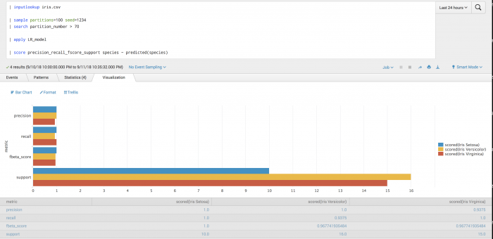


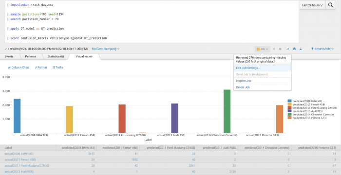
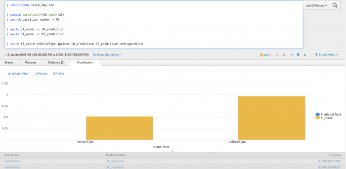
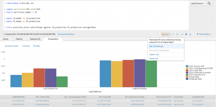
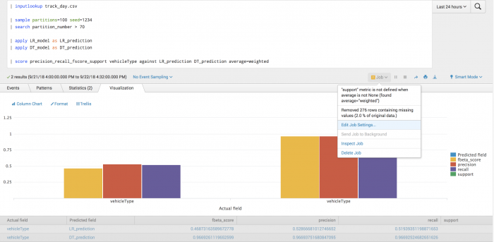
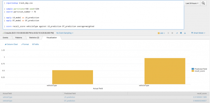

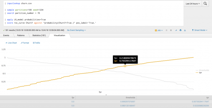


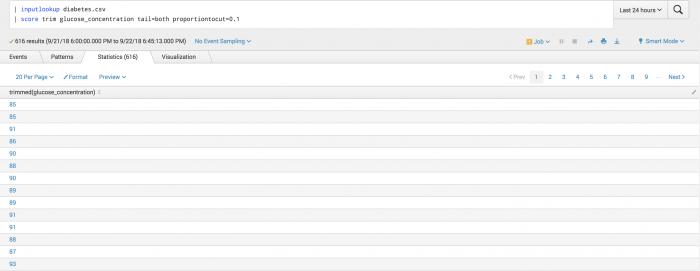


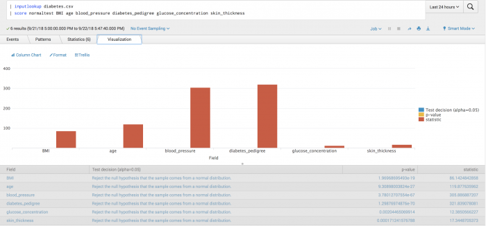


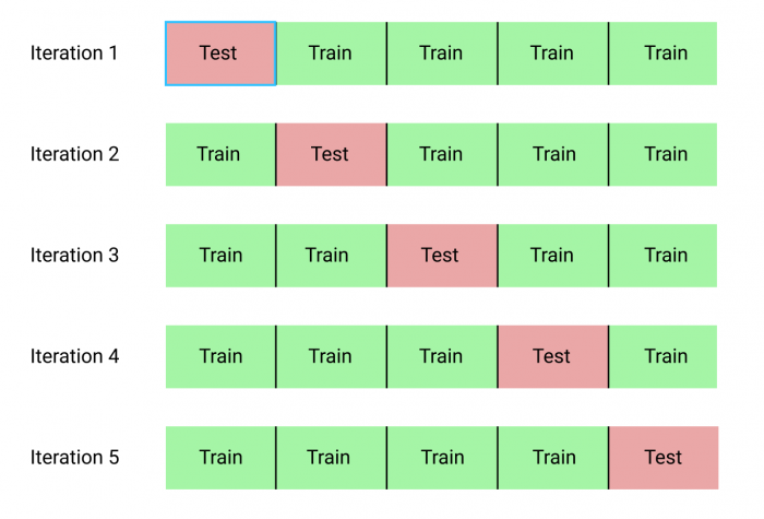


 Download manual
Feedback submitted, thanks!