Predict Numeric Fields

The Predict Numeric Fields assistant performs a prediction on numeric values, using an algorithm commonly called Linear Regression, which fits a line to the data. Such models are useful for determining to what extent certain peripheral factors contribute to a particular metric result. Once the regression model is computed, you can use these peripheral values to make a prediction on the metric result.

Algorithm

• Linear Regression

Workflow

To predict numeric fields, you must fit and train a model. The basic steps are as follows:

1. Enter a search to retrieve your data, then click the search button to run it.
2. Select the numeric field you want to predict. This list of fields is populated by the search you just ran.
3. Select a combination of fields you want to use for predicting the numeric field. This list contains all of the fields from your search except for the field you selected to predict.
4. Specify how much of your data to use for training (fitting the data model) versus testing (validating the model afterwards). The data is divided randomly into two groups. The default split is 50/50.
5. Name the model. This name and the settings you select are saved in the history in the Load Existing Settings tab.
6. Click Fit Model.

Interpret and validate

After you fit the model, review the prediction results and visualizations to see how well the model predicted the numeric field.

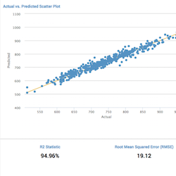
• Actual vs. Predicted Scatter Plot: Shows the predicted value (the yellow line) against the raw actual values (blue dots) for the field you chose to predict. Hover on the blue dots to see actual values.

Interpretation: The yellow line showing the "perfect" result generally isn't attainable, but the closer the points are to the line, the better the model.

• Residuals Histogram: Displays a histogram of the difference between the actual values (the yellow line) and the predicted values (the blue bars). Hover over the blue bars to see the residual error (different between the actual and predicted result) and sample count (the number of results with this error).

Interpretation: In a perfect world all the residuals would be zero. In reality, the residuals probably end on a bell curve that is ideally clustered tightly around zero.

• R² Statistic: Explains how well the model explains the variability of the result. 100% (a value of 1) means the model fits perfectly.

Interpretation: The closer the value is to 1 (100%), the better the result.

• Root Mean Squared Error: Explains the variability of the result, which is essentially the standard deviation of the residual. The formula takes the difference between actual and predicted values, squares this value, takes an average, and then takes a square root.

Interpretation: This value can be arbitrarily large and just gives you an idea of how close or far the model is. These values only make sense within one dataset and shouldn’t be compared across datasets.

• Fit Model Parameters Summary: Displays the coefficients associated with each variable in the regression model. A relatively high coefficient value shows a high association of that variable with the result. A negative value shows a negative correlation.
• Actual vs. Predicted Overlay: Shows the actual values against the predicted values, in sequence.
• Residuals: Shows the residual (difference between predicted and actual) values, in sequence.

Refine the model

After you have validated the model, the way to refine the model is by adjusting which fields you use to predict the numeric field and fit the model again:

• Remove fields that might generate a distraction.
• Try adding more fields. In the Load Existing Settings tab, which displays a history of models you have fitted, sort by the R² statistic to see which combination of fields yielded the best results.

Deploy the model

Once you have validated and refined a model and are satisfied with it, you can take the following actions:

• Click the icon in the right part of the Fit Model button to schedule model training. You can set up a regular interval to fit the model, such as every week. After saving the schedule, you can access it from the Scheduled Jobs > Scheduled Training menu.
• Click the Open in Search button next to the Fit Model button to open a new Search tab, filled out with a search query that uses all data (not just the training set).
• Click the Show SPL button next to the Open in Search button to see the search query that was used to fit the model. For example, you could use this same query on a different data set.
• Click the Schedule Alert button beneath the Prediction Results table to trigger an alert when the predicted value meets a threshold you specify. After you save the alert, you can access it from the Scheduled Jobs > Alerts menu.