Aggregate functions
Aggregate functions summarize the values from each event to create a single, meaningful value. Common aggregate functions include Average, Count, Minimum, Maximum, Standard Deviation, Sum, and Variance.
Most aggregate functions are used with numeric fields. However, there are some functions that you can use with either alphabetic string fields or numeric fields. The function descriptions indicate which functions you can use with alphabetic strings.
For an overview, see statistical and charting functions.
avg(<value>)
Description
Returns the average of the values of the field specified.
Usage
You can use this function with the chart, mstats, stats, timechart, and tstats commands, and also with sparkline() charts.
For a list of the related statistical and charting commands that you can use with this function, see Statistical and charting functions.
Basic examples
Example 1
The following example returns the average (mean) "size" for each distinct "host".
... | stats avg(size) BY host
Example 2
The following example returns the average "thruput" of each "host" for each 5 minute time span.
... | bin _time span=5m | stats avg(thruput) BY _time host
Example 3
The following example charts the ratio of the average (mean) "size" to the maximum "delay" for each distinct "host" and "user" pair.
... | chart eval(avg(size)/max(delay)) AS ratio BY host user
Example 4
The following example displays a timechart of the average of cpu_seconds by processor, rounded to 2 decimal points.
... | timechart eval(round(avg(cpu_seconds),2)) BY processor
Extended examples
Example 1
There are situations where the results of a calculation can return a different accuracy to the very far right of the decimal point. For example, the following search calculates the average of 100 values:
| makeresults count=100 | eval test=3.99 | stats avg(test)
The result of this calculation is:
| avg(test) |
|---|
| 3.9900000000000055 |
When the count is changed to 10000, the results are different:
| makeresults count=10000 | eval test=3.99 | stats avg(test)
The result of this calculation is:
| avg(test) |
|---|
| 3.990000000000215 |
This occurs because numbers are treated as double-precision floating-point numbers.
To mitigate this issue, you can use the sigfig function to specify the number of significant figures you want returned.
However, first you need to make a change to the stats command portion of the search. You need to change the name of the field avg(test) to remove the parenthesis. For example stats avg(test) AS test. The sigfig function expects either a number or a field name. The sigfig function cannot accept a field name that looks like another function, in this case avg.
To specify the number of decimal places you want returned, you multiply the field name by 1 and use zeros to specify the number of decimal places. If you want 4 decimal places returned, you would multiply the field name by 1.0000. To return 2 decimal places, multiply by 1.00, as shown in the following example:
| makeresults count=10000 | eval test=3.99 | stats avg(test) AS test | eval new_test=sigfig(test*1.00)
The result of this calculation is:
| test |
|---|
| 3.99 |
Example 2
Chart the average number of events in a transaction, based on transaction duration.
| This example uses the sample data from the Search Tutorial. To try this example on your own Splunk instance, you must download the sample data and follow the instructions to get the tutorial data into Splunk. Use the time range All time when you run the search. |
-
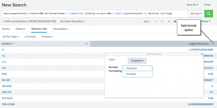
Run the following search to create a chart to show the average number of events in a transaction based on the duration of the transaction.
sourcetype=access_* status=200 action=purchase | transaction clientip maxspan=30m | chart avg(eventcount) by duration span=log2The
transactioncommand adds two fields to the resultsdurationandeventcount. Theeventcountfield tracks the number of events in a single transaction.In this search, the transactions are piped into the
chartcommand. Theavg()function is used to calculate the average number of events for each duration. Because the duration is in seconds and you expect there to be many values, the search uses thespanargument to bucket the duration into bins using logarithm with a base of 2. - Use the field format option to enable number formatting.
- Click the Visualization tab and change the display to a pie chart.
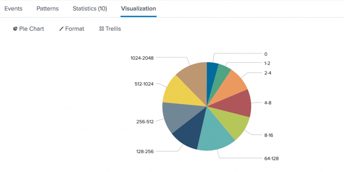
Each wedge of the pie chart represents a duration for the event transactions. You can hover over a wedge to see the average values.


count(<value>) or c(<value>)
Description
Returns the number of occurrences of the field specified. To indicate a specific field value to match, format <value> as eval(field="value"). Processes field values as strings. To use this function, you can specify count(<value>), or the abbreviation c(<value>).
Usage
You can use this function with the chart, mstats, stats, timechart, and tstats commands, and also with sparkline() charts.
Basic examples
The following example returns the count of events where the status field has the value "404".
...| stats count(eval(status="404")) AS count_status BY sourcetype
This example uses an eval expression with the count function. See Using eval expressions in stats functions.
The following example separates search results into 10 bins and returns the count of raw events for each bin.
... | bin size bins=10 | stats count(_raw) BY size
The following example generates a sparkline chart to count the events that use the _raw field.
... sparkline(count)
The following example generates a sparkline chart to count the events that have the user field.
... sparkline(count(user))
The following example uses the timechart command to count the events where the action field contains the value purchase.
sourcetype=access_* | timechart count(eval(action="purchase")) BY productName usenull=f useother=f
Extended examples
Count the number of earthquakes that occurred for each magnitude range
| This search uses recent earthquake data downloaded from the USGS Earthquakes website. The data is a comma separated ASCII text file that contains magnitude (mag), coordinates (latitude, longitude), region (place), etc., for each earthquake recorded.
You can download a current CSV file from the USGS Earthquake Feeds and upload the file to your Splunk instance. This example uses the All Earthquakes data from the past 30 days. |
- Run the following search to calculate the number of earthquakes that occurred in each magnitude range. This data set is comprised of events over a 30-day period.
source=all_month.csv | chart count AS "Number of Earthquakes" BY mag span=1 | rename mag AS "Magnitude Range"- This search uses
span=1to define each of the ranges for the magnitude field,mag. - The rename command is then used to rename the field to "Magnitude Range".
The results look something like this:Magnitude Range Number of Earthquakes -1-0 18 0-1 2088 1-2 3005 2-3 1026 3-4 194 4-5 452 5-4 109 6-7 11 7-8 3 - This search uses
Count the number of different page requests for each Web server
| This example uses the sample data from the Search Tutorial but should work with any format of Apache web access log. To try this example on your own Splunk instance, you must download the sample data and follow the instructions to get the tutorial data into Splunk. Use the time range All time when you run the search. |
-
Run the following search to use the
chartcommand to determine the number of different page requests, GET and POST, that occurred for each Web server.sourcetype=access_* | chart count(eval(method="GET")) AS GET, count(eval(method="POST")) AS POST BY hostThis example uses
evalexpressions to specify the different field values for thestatscommand to count. The first clause uses thecount()function to count the Web access events that contain themethodfield valueGET. Then, using the AS keyword, the field that represents these results is renamed GET.The second clause does the same for POST events. The counts of both types of events are then separated by the web server, using the BY clause with the
hostfield.The results appear on the Statistics tab and look something like this:
host GET POST www1 8431 5197 www2 8097 4815 www3 8338 465 -
Click the Visualization tab. If necessary, format the results as a column chart. This chart displays the total count of events for each event type, GET or POST, based on the
hostvalue.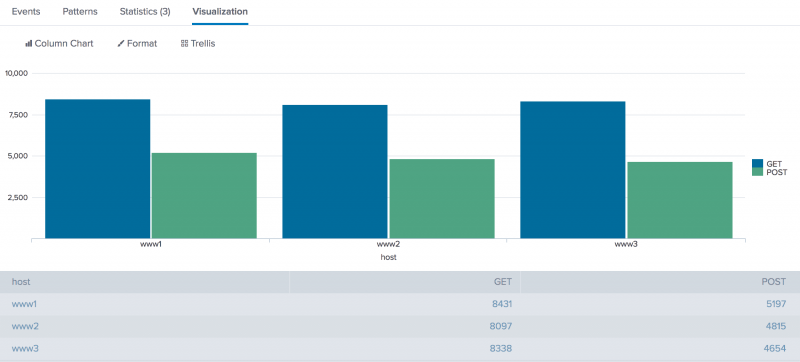

distinct_count(<value>) or dc(<value>)
Description
Returns the count of distinct values of the field specified. This function processes field values as strings. To use this function, you can specify distinct_count(<value>), or the abbreviation dc(<value>).
Usage
You can use this function with the chart, mstats, stats, timechart, and tstats commands, and also with sparkline() charts.
Basic examples
The following example removes duplicate results with the same "host" value and returns the total count of the remaining results.
... | stats dc(host)
The following example generates sparklines for the distinct count of devices and renames the field, "numdevices".
...sparkline(dc(device)) AS numdevices
The following example counts the distinct sources for each sourcetype, and buckets the count for each five minute spans.
...sparkline(dc(source),5m) BY sourcetype
Extended example
| This example uses the sample data from the Search Tutorial. To try this example on your own Splunk instance, you must download the sample data and follow the instructions to get the tutorial data into Splunk. Use the time range Yesterday when you run the search. |
- Run the following search to count the number of different customers who purchased something from the Buttercup Games online store yesterday. The search organizes the count by the type of product (accessories, t-shirts, and type of games) that customers purchased.
sourcetype=access_* action=purchase | stats dc(clientip) BY categoryId- This example first searches for purchase events,
action=purchase. - These results are piped into the
statscommand and thedc()function counts the number of different users who make purchases. - The
BYclause is used to break up this number based on the different category of products, thecategoryId.
The results appear on the Statistics tab and look something like this:categoryId dc(clientip) ACCESSORIES 37 ARCADE 58 NULL 8 SHOOTER 31 SIMULATION 34 SPORTS 13 STRATEGY 74 TEE 38 - This example first searches for purchase events,
estdc(<value>)
Description
Returns the estimated count of the distinct values of the field specified. This function processes field values as strings. The string values 1.0 and 1 are considered distinct values and counted separately.
Usage
You can use this function with the chart, stats, timechart, and tstats commands.
By default, if the actual number of distinct values returned by a search is below 1000, the Splunk software does not estimate the distinct value count for the search. It uses the actual distinct value count instead. This threshold is set by the approx_dc_threshold setting in limits.conf.
Basic examples
The following example removes duplicate results with the same "host" value and returns the estimated total count of the remaining results.
... | stats estdc(host)
The results look something like this:
| estdc(host) |
|---|
| 6 |
The following example generates sparklines for the estimated distinct count of the devices field and renames the results field, "numdevices".
...sparkline(estdc(device)) AS numdevices
The following example estimates the distinct count for the sources for each sourcetype. The results are displayed for each five minute span in sparkline charts.
...sparkline(estdc(source),5m) BY sourcetype
estdc_error(<value>)
Description
Returns the theoretical error of the estimated count of the distinct values of the field specified. The error represents a ratio of the absolute_value(estimate_distinct_count - real_distinct_count)/real_distinct_count. This function processes field values as strings.
Usage
You can use this function with the chart, stats, and timechart commands.
Basic examples
The following example determines the error ratio for the estimated distinct count of the "host" values.
... | stats estdc_error(host)
exactperc<percentile>(<value>)
Description
Returns a percentile value of the numeric field specified.
Usage
You can use this function with the chart, stats, timechart, and tstats commands, and also with sparkline() charts.
The exactperc function provides the exact value, but is very resource expensive for high cardinality fields. The exactperc function can consume a large amount of memory in the search head, which might impact how long it takes for a search to complete.
Examples
See the perc<percentile>(<value>) function.
max(<value>)
Description
Returns the maximum value of the field specified. If the values in the field are non-numeric, the maximum value is found using lexicographical ordering.
Processes field values as numbers if possible, otherwise processes field values as strings.
Usage
You can use this function with the chart, mstats, stats, and timechart commands, and also with sparkline() charts.
Lexicographical order sorts items based on the values used to encode the items in computer memory. In Splunk software, this is almost always UTF-8 encoding, which is a superset of ASCII.
- If the items are all numeric, they're sorted in numerical order based on the first digit. For example, the numbers 10, 9, 70, 100 are sorted as 10, 100, 70, 9.
- if the items are mixed, they're sorted in numeric and then lexicographical order with all numbers sorted before non-numeric items. For example, the items 1, c, a, 2, 100, b, 4, 9 are sorted as 1, 2, 4, 9, 100, a, b, c.
- if all items are non-numeric, they're sorted in lexicographical order.
- Uppercase letters are sorted before lowercase letters.
- Symbols are not standard. Some symbols are sorted before numeric values. Other symbols are sorted before or after letters.
Basic examples
This example returns the maximum value of the size field.
... | stats max(size)
Extended example
Calculate aggregate statistics for the magnitudes of earthquakes in an area
| This search uses recent earthquake data downloaded from the USGS Earthquakes website. The data is a comma separated ASCII text file that contains magnitude (mag), coordinates (latitude, longitude), region (place), etc., for each earthquake recorded.
You can download a current CSV file from the USGS Earthquake Feeds and upload the file to your Splunk instance. This example uses the All Earthquakes data from the past 30 days. |
- Search for earthquakes in and around California. Calculate the number of earthquakes that were recorded. Use statistical functions to calculate the minimum, maximum, range (the difference between the min and max), and average magnitudes of the recent earthquakes. List the values by magnitude type.
source=all_month.csv place=*California* | stats count, max(mag), min(mag), range(mag), avg(mag) BY magTypeThe results appear on the Statistics tab and look something like this:
magType count max(mag) min(mag) range(mag) avg(mag) H 123 2.8 0.0 2.8 0.549593 MbLg 1 0 0 0 0.0000000 Md 1565 3.2 0.1 3.1 1.056486 Me 2 2.0 1.6 .04 1.800000 Ml 1202 4.3 -0.4 4.7 1.226622 Mw 6 4.9 3.0 1.9 3.650000 ml 10 1.56 0.19 1.37 0.934000
mean(<value>)
Description
Returns the arithmetic mean of the field specified.
The mean values should be exactly the same as the values calculated using the avg() function.
Usage
You can use this function with the chart, mstats, stats, and timechart commands, and also with sparkline() charts.
Basic examples
The following example returns the mean of "kbps" values:
... | stats mean(kbps)
Extended example
| This search uses recent earthquake data downloaded from the USGS Earthquakes website. The data is a comma separated ASCII text file that contains magnitude (mag), coordinates (latitude, longitude), region (place), etc., for each earthquake recorded.
You can download a current CSV file from the USGS Earthquake Feeds and upload the file to your Splunk instance. This example uses the All Earthquakes data from the past 30 days. |
-
Run the following search to find the mean, standard deviation, and variance of the magnitudes of recent quakes by magnitude type.
source=usgs place=*California* | stats count mean(mag), stdev(mag), var(mag) BY magTypeThe results look something like this:
magType count mean(mag) std(mag) var(mag) H 123 0.549593 0.356985 0.127438 MbLg 1 0.000000 0.000000 0.000000 Md 1565 1.056486 0.580042 0.336449 Me 2 1.800000 0.346410 0.120000 Ml 1202 1.226622 0.629664 0.396476 Mw 6 3.650000 0.716240 0.513000 ml 10 0.934000 0.560401 0.314049
median(<value>)
Description
Returns the middle-most value of the field specified.
Usage
You can use this function with the chart, mstats, stats, and timechart commands.
If you have an even number of events, by default the median calculation is approximated to the higher of the two values.
This function is, by its nature, nondeterministic. This means that subsequent runs of a search using this function over identical data can contain slight variances in their results.
If you require results that are more exact and consistent you can use exactperc50() instead. However, the exactperc<percentile>(<value>) function is very resource expensive for high cardinality fields. See perc<percentile>(<value>).
Basic examples
Consider the following list of values, which counts the number of different customers who purchased something from the Buttercup Games online store yesterday. The values are organized by the type of product (accessories, t-shirts, and type of games) that customers purchased.
| categoryId | count |
|---|---|
| ACCESSORIES | 37 |
| ARCADE | 58 |
| NULL | 8 |
| SIMULATION | 34 |
| SPORTS | 13 |
| STRATEGY | 74 |
| TEE | 38 |
When the list is sorted the median, or middle-most value, is 37.
| categoryId | count |
|---|---|
| NULL | 8 |
| SPORTS | 13 |
| SIMULATION | 34 |
| ACCESSORIES | 37 |
| TEE | 38 |
| ARCADE | 58 |
| STRATEGY | 74 |
min(<value>)
Description
Returns the minimum value of the field specified. If the values of X are non-numeric, the minimum value is found using lexicographical ordering.
This function processes field values as numbers if possible, otherwise processes field values as strings.
Usage
You can use this function with the chart, mstats, stats, and timechart commands.
Lexicographical order sorts items based on the values used to encode the items in computer memory. In Splunk software, this is almost always UTF-8 encoding, which is a superset of ASCII.
- If the items are all numeric, they're sorted in numerical order based on the first digit. For example, the numbers 10, 9, 70, 100 are sorted as 10, 100, 70, 9.
- If the items are mixed, they're sorted in numeric and then lexicographical order with all numbers sorted before non-numeric items. For example, the items 1, c, a, 2, 100, b, 4, 9 are sorted as 1, 2, 4, 9, 100, a, b, c.
- If all items are non-numeric, they're sorted in lexicographical order.
- Uppercase letters are sorted before lowercase letters.
- Symbols are not standard. Some symbols are sorted before numeric values. Other symbols are sorted before or after letters.
Basic examples
The following example returns the minimum size and maximum size of the HotBucketRoller component in the _internal index.
index=_internal component=HotBucketRoller | stats min(size), max(size)
The following example returns a list of processors and calculates the minimum cpu_seconds and the maximum cpu_seconds.
index=_internal | chart min(cpu_seconds), max(cpu_seconds) BY processor
Extended example
See the Extended example for the max() function. That example includes the min() function.
mode(<value>)
Description
Returns the most frequent value of the field specified.
Processes field values as strings.
Usage
You can use this function with the chart, stats, and timechart commands.
Basic examples
The mode returns the most frequent value. Consider the following data:
| firstname | surname | age |
|---|---|---|
| Claudia | Garcia | 32 |
| David | Mayer | 45 |
| Alex | Garcia | 29 |
| Wei | Zhang | 45 |
| Javier | Garcia | 37 |
When you search for the mode in the age field, the value 45 is returned.
...| stats mode(age)
You can also use mode with fields that contain string values. When you search for the mode in the surname field, the value Garcia is returned.
...| stats mode(surname)
Here's another set of sample data:
| _time | host | sourcetype |
|---|---|---|
| 04-06-2020 17:06:23.000 PM | www1 | access_combined |
| 04-06-2020 10:34:19.000 AM | www1 | access_combined |
| 04-03-2020 13:52:18.000 PM | www2 | access_combined |
| 04-02-2020 07:39:59.000 AM | www3 | access_combined |
| 04-01-2020 19:35:58.000 PM | www1 | access_combined |
If you run a search that looks for the mode in the host field, the value www1 is returned because it is the most common value in the host field. For example:
... |stats mode(host)
The results look something like this:
| mode(host) |
|---|
| www1 |
perc<percentile>(<value>)
Description
The percentile functions return the Nth percentile value of the numeric field <value>. You can think of this as an estimate of where the top percentile starts. For example, a 95th percentile says that 95% of the values in field Y are below the estimate and 5% of the values in field <value> are above the estimate.
Valid percentile values are floating point numbers between 0 and 100, such as 99.95.
There are three different percentile functions that you can use:
| Function | Description |
|---|---|
| perc<percentile>(<value>) or the abbreviation p<percentile>(<value>) | Use the perc function to calculate an approximate threshold, such that of the values in field Y, X percent fall below the threshold. The perc function returns a single number that represents the lower end of the approximate values for the percentile requested.
|
| upperperc<percentile>(<value>) | When there are more than 1000 values, the upperperc function gives the approximate upper bound for the percentile requested. Otherwise the upperperc function returns the same percentile as the perc function.
|
| exactperc<percentile>(<value>) | The exactperc function provides the exact value, but is very resource expensive for high cardinality fields. The exactperc function can consume a large amount of memory, which might impact how long it takes for a search to complete.
|
The percentile functions process field values as strings.
The perc and upperperc functions are, by their nature, nondeterministic, which means that that subsequent runs of searches using these functions over identical data can contain slight variances in their results.
If you require exact and consistent results, you can use exactperc<X>(Y) instead.
Usage
You can use this function with the chart, mstats, stats, timechart, and tstats commands.
Differences between Splunk and Excel percentile algorithms
If there are less than 1000 distinct values, the Splunk percentile functions use the nearest rank algorithm. See http://en.wikipedia.org/wiki/Percentile#Nearest_rank. Excel uses the NIST interpolated algorithm, which basically means you can get a value for a percentile that does not exist in the actual data, which is not possible for the nearest rank approach.
Splunk algorithm with more than 1000 distinct values
If there are more than 1000 distinct values for the field, the percentiles are approximated using a custom radix-tree digest-based algorithm. This algorithm is much faster and uses much less memory, a constant amount, than an exact computation, which uses memory in linear relation to the number of distinct values. By default this approach limits the approximation error to < 1% of rank error. That means if you ask for 95th percentile, the number you get back is between the 94th and 96th percentile.
You always get the exact percentiles even for more than 1000 distinct values by using the exactperc function compared to the perc.
Basic examples
Consider this list of values Y = {10,9,8,7,6,5,4,3,2,1}.
The following example returns 5.5.
...| stats perc50(Y)
The following example returns 9.55.
...| stats perc95(Y)
Extended example
Consider the following set of data, which shows the number of visitors for each hour a store is open:
| hour | visitors |
|---|---|
| 0800 | 0 |
| 0900 | 212 |
| 1000 | 367 |
| 1100 | 489 |
| 1200 | 624 |
| 1300 | 609 |
| 1400 | 492 |
| 1500 | 513 |
| 1600 | 376 |
| 1700 | 337 |
This data resides in the visitor_count index. You can use the streamstats command to create a cumulative total for the visitors.
index=visitor_count | streamstats sum(visitors) as 'visitors total'
The results from this search look like this:
| hour | visitors | visitors total |
|---|---|---|
| 0800 | 0 | 0 |
| 0900 | 212 | 212 |
| 1000 | 367 | 579 |
| 1100 | 489 | 1068 |
| 1200 | 624 | 1692 |
| 1300 | 609 | 2301 |
| 1400 | 492 | 2793 |
| 1500 | 513 | 3306 |
| 1600 | 376 | 3673 |
| 1700 | 337 | 4010 |
Let's add the stats command with the perc function to determine the 50th and 95th percentiles.
index=visitor_count | streamstats sum(visitors) as 'visitors total' | stats perc50('visitors total') perc95('visitors total')
The results from this search look like this:
| perc50(visitors total) | perc95(visitors total) |
|---|---|
| 1996.5 | 3858.35 |
The perc50 estimates the 50th percentile, when 50% of the visitors had arrived. You can see from the data that the 50th percentile was reached between visitor number 1996 and 1997, which was sometime between 1200 and 1300 hours. The perc95 estimates the 95th percentile, when 95% of the visitors had arrived. The 95th percentile was reached with visitor 3858, which occurred between 1600 and 1700 hours.
range(<value>)
Description
Returns the difference between the max and min values of the field specified. The values in the field must be numeric.
Usage
You can use this function with the chart, mstats, stats, timechart, and tstats commands, and also with sparkline() charts.
Basic example
This example uses events that list the numeric sales for each product and quarter, for example:
| products | quarter | sales | quota |
|---|---|---|---|
| ProductA | QTR1 | 1200 | 1000 |
| ProductB | QTR1 | 1400 | 1550 |
| ProductC | QTR1 | 1650 | 1275 |
| ProductA | QTR2 | 1425 | 1300 |
| ProductB | QTR2 | 1175 | 1425 |
| ProductC | QTR2 | 1550 | 1450 |
| ProductA | QTR3 | 1300 | 1400 |
| ProductB | QTR3 | 1250 | 1125 |
| ProductC | QTR3 | 1375 | 1475 |
| ProductA | QTR4 | 1550 | 1300 |
| ProductB | QTR4 | 1700 | 1225 |
| ProductC | QTR4 | 1625 | 1350 |
It is easiest to understand the range if you also determine the min and max values. To determine the range of sales by product, run this search:
source="addtotalsData.csv" | chart sum(sales) min(sales) max(sales) range(sales) BY products
The results look something like this:
| quarter | sum(sales) | min(sales) | max(sales) | range(sales) |
|---|---|---|---|---|
| QTR1 | 4250 | 1200 | 1650 | 450 |
| QTR2 | 4150 | 1175 | 1550 | 375 |
| QTR3 | 3925 | 1250 | 1375 | 125 |
| QTR4 | 4875 | 1550 | 1700 | 150 |
The range(sales) is the max(sales) minus the min(sales).
Extended example
See the Extended example for the max() function. That example includes the range() function.
stdev(<value>)
Description
Returns the sample standard deviation of the field specified.
Usage
You can use this function with the chart, mstats, stats, timechart, and tstats commands, and also with sparkline() charts.
Basic examples
This example returns the standard deviation of wildcarded fields "*delay" which can apply to both, "delay" and "xdelay".
... | stats stdev(*delay)
Extended example
| This search uses recent earthquake data downloaded from the USGS Earthquakes website. The data is a comma separated ASCII text file that contains magnitude (mag), coordinates (latitude, longitude), region (place), etc., for each earthquake recorded.
You can download a current CSV file from the USGS Earthquake Feeds and upload the file to your Splunk instance. This example uses the All Earthquakes data from the past 30 days. |
-
Run the following search to find the mean, standard deviation, and variance of the magnitudes of recent quakes by magnitude type.
source=usgs place=*California* | stats count mean(mag), stdev(mag), var(mag) BY magTypeThe results look something like this:
magType count mean(mag) std(mag) var(mag) H 123 0.549593 0.356985 0.127438 MbLg 1 0.000000 0.000000 0.000000 Md 1565 1.056486 0.580042 0.336449 Me 2 1.800000 0.346410 0.120000 Ml 1202 1.226622 0.629664 0.396476 Mw 6 3.650000 0.716240 0.513000 ml 10 0.934000 0.560401 0.314049
stdevp(<value>)
Description
Returns the population standard deviation of the field specified.
Usage
You can use this function with the chart, mstats, stats, timechart, and tstats commands, and also with sparkline() charts.
Basic examples
Extended example
sum(<value>)
Description
Returns the sum of the values of the field specified.
Usage
You can use this function with the chart, mstats, stats, timechart, and tstats commands, and also with sparkline() charts.
Basic examples
You can create totals for any numeric field. For example:
...| stats sum(bytes)
The results look something like this:
| sum(bytes) |
|---|
| 21502 |
You can rename the column using the AS keyword:
...| stats sum(bytes) AS "total bytes"
The results look something like this:
| total bytes |
|---|
| 21502 |
You can organize the results using a BY clause:
...| stats sum(bytes) AS "total bytes" by date_hour
The results look something like this:
| date_hour | total bytes |
|---|---|
| 07 | 6509 |
| 11 | 3726 |
| 15 | 6569 |
| 23 | 4698 |
sumsq(<value>)
Description
Returns the sum of the squares of the values of the field specified.
The sum of the squares is used to evaluate the variance of a dataset from the dataset mean. A large sum of the squares indicates a large variance, which tells you that individual values fluctuate widely from the mean.
Usage
You can use this function with the chart, mstats, stats, timechart, and tstats commands, and also with sparkline() charts.
Basic examples
The following table contains the temperatures taken every day at 8 AM for a week.
You calculate the mean of the these temperatures and get 48.9 degrees. To calculate the deviation from the mean for each day, take the temperature and subtract the mean. If you square each number, you get results like this:
| day | temp | mean | deviation | square of temperatures |
|---|---|---|---|---|
| sunday | 65 | 48.9 | 16.1 | 260.6 |
| monday | 42 | 48.9 | -6.9 | 47.0 |
| tuesday | 40 | 48.9 | -8.9 | 78.4 |
| wednesday | 31 | 48.9 | -17.9 | 318.9 |
| thursday | 47 | 48.9 | -1.9 | 3.4 |
| friday | 53 | 48.9 | 4.1 | 17.2 |
| saturday | 64 | 48.9 | 15.1 | 229.3 |
Take the total of the squares, 954.9, and divide by 6 which is the number of days minus 1. This gets you the sum of squares for this series of temperatures. The standard deviation is the square root of the sum of the squares. The larger the standard deviation the larger the fluctuation in temperatures during the week.
You can calculate the mean, sum of the squares, and standard deviation with a few statistical functions:
...|stats mean(temp), sumsq(temp), stdev(temp)
This search returns these results:
| mean(temp) | sumsq(temp) | stdev(temp) |
|---|---|---|
| 48.857142857142854 | 17664 | 12.615183595289349 |
upperperc<percentile>(<value>)
Description
Returns an approximate percentile value, based on the requested percentile of the numeric field.
When there are more than 1000 values, the upperperc function gives the approximate upper bound for the percentile requested. Otherwise the upperperc function returns the same percentile as the perc function.
See the percentile<percentile>(<value>) function.
Usage
You can use this function with the chart, mstats, stats, timechart, and tstats commands, and also with sparkline() charts.
Examples
See the perc function.
var(<value>)
Description
Returns the sample variance of the field specified.
Usage
You can use this function with the chart, mstats, stats, timechart, and tstats commands, and also with sparkline() charts.
Example
See the Extended example for the mean() function. That example includes the var() function.
varp(<value>)
Description
Returns the population variance of the field specified.
Usage
You can use this function with the chart, mstats, stats, timechart, and tstats commands, and also with sparkline() charts.
Basic examples
| Statistical and charting functions | Event order functions |
This documentation applies to the following versions of Splunk® Enterprise: 7.1.0, 7.1.1, 7.1.2, 7.1.3, 7.1.4, 7.1.5, 7.1.6, 7.1.7, 7.1.8, 7.1.9, 7.1.10, 7.2.0, 7.2.1, 7.2.2, 7.2.3, 7.2.4, 7.2.5, 7.2.6, 7.2.7, 7.2.8, 7.2.9, 7.2.10, 7.3.0, 7.3.1, 7.3.2, 7.3.3, 7.3.4, 7.3.5, 7.3.6, 7.3.7, 7.3.8, 7.3.9, 8.0.0, 8.0.1, 8.0.2, 8.0.3, 8.0.4, 8.0.5, 8.0.6, 8.0.7, 8.0.8, 8.0.9, 8.0.10, 8.1.0, 8.1.1, 8.1.2, 8.1.3, 8.1.4, 8.1.5, 8.1.6, 8.1.7, 8.1.8, 8.1.9, 8.1.10, 8.1.11, 8.1.12, 8.1.13, 8.1.14, 8.2.0, 8.2.1, 8.2.2, 8.2.3, 8.2.4, 8.2.5, 8.2.6, 8.2.7, 8.2.8, 8.2.9, 8.2.10, 8.2.11, 8.2.12, 9.0.0, 9.0.1, 9.0.2, 9.0.3, 9.0.4, 9.0.5, 9.0.6, 9.0.7, 9.0.8, 9.0.9, 9.0.10, 9.1.0, 9.1.1, 9.1.2, 9.1.3, 9.1.4, 9.1.5, 9.1.6, 9.1.7, 9.1.8, 9.1.9, 9.2.0, 9.2.1, 9.2.2, 9.2.3, 9.2.4, 9.2.5, 9.2.6, 9.3.0, 9.3.1, 9.3.2, 9.3.3, 9.3.4, 9.4.0, 9.4.1, 9.4.2
Feedback submitted, thanks!