Train a predictive model in ITSI
The process of training a predictive model in IT Service Intelligence (ITSI) involves providing a machine learning algorithm with training data to learn from. The term "model" refers to the model artifact created by the training process. The learning algorithm finds patterns in the training data and produces a machine learning model that captures these patterns.
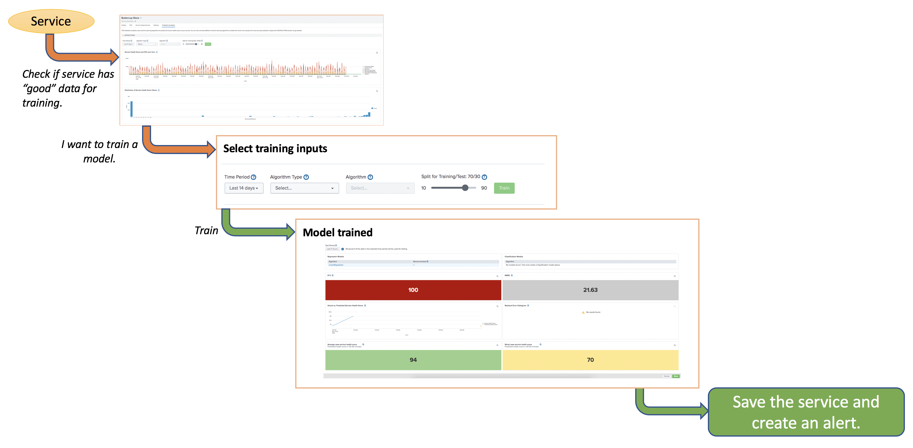
To train a predictive model for a service, go to the Predictive Analytics tab of the service and perform the following steps:
- Specify a time period.
- Choose an algorithm type.
- Choose a machine learning algorithm.
- Split your data into training and test sets.
After you train the model, you can save it into the service and create an alert that notifies you of potential service degradation.
The following diagram shows the high-level workflow for training a model:
If you have a lot of data in the summary index, the process of training a model can take up to 30 minutes to complete. During this training period, do not navigate away from the page.
Prerequisites
To train a model, you first need to decide whether the data for the selected service is a good fit for predictive modeling. For instructions, see Determine whether your service is a good fit for modeling in ITSI.
Specify a time period
The time period determines how far back ITSI looks when training a predictive model. The amount of data a predictive model needs depends on the complexity and shape of your data within the time period, and the complexity of the algorithm.
Consider the following guidelines when you choose a time period:
- Use at least 14 days of data. 30 days or more is recommended.
- In general, a model needs enough data to reasonably capture the relationships that exist among inputs (past KPI values and service health scores) and between inputs and outputs (future service health scores).
- To encapsulate as much variance in your data as possible, use as much data as you have available to train a model. It's best to operate under the assumption that the more data you provide, the better.
If you don't have enough data in the summary index to adequately train a model, consider backfilling the summary index with service health score data. For more information, see Backfill service health scores in ITSI.
To look more closely at the shape and complexity of your data, consult the following graphs:
Choose an algorithm type
There are two types of algorithms you can use to train predictive models in ITSI: regression and classification. Fundamentally, regression is about predicting a numerical service health score, and classification is about predicting a service health state.
Regression algorithms
Regression algorithms predict numeric values. For example, salary or age. In ITSI Predictive Analytics, regression algorithms predict an actual numeric health score value (for example, health score=89). Such models are useful for determining to what extent peripheral factors, such as historical KPI values, contribute to a particular metric result (service health score). After the regression model is computed, you can use these peripheral values to make a prediction on the metric result.
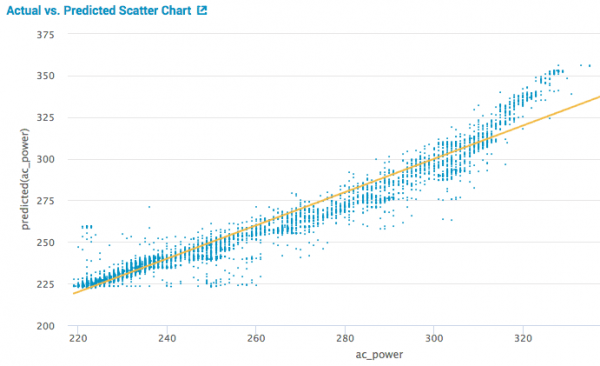
The following visualization illustrates a scatter plot of actual versus predicted results. The test data is plotted, and the yellow line indicates the best fit line for predicting server power consumption.
Classification algorithms
A classification algorithm predicts a category. For example, diabetic or not diabetic, rather than a discrete numeric value such as cholesterol levels. The algorithm learns the tendency for data to belong to one category or another based on related data. In ITSI Predictive Analytics, a classification algorithm uses the training data to predict a service health state (Normal, Medium, or Critical).
In short, classification classifies data and constructs a model based on the training set, and uses that model in classifying new data.
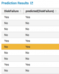
For example, the following classification table shows the actual state of a field versus the predicted state of the field. The yellow bar highlights an incorrect prediction.
Choose a machine learning algorithm
ITSI provides the following machine learning algorithms:
- Linear regression (Regression)
- Random forest regressor (Regression)
- Gradient boosting regressor (Regression)
- Logistic regression (Classification)
Linear regression
The linear regression algorithm creates a model for the relationship between multiple independent input variables (historical KPI and service health score values) and an output dependent variable (future service health score). The model remains linear in the sense that the output is a linear combination of the input variables. The algorithm learns by estimating the coefficient values in the test set using the data available in the training set.
| Strengths | Weaknesses |
|---|---|
| Useful when the relationship to be modeled is not extremely complex and if you don't have a lot of data. | Tends to underperform when there are multiple or non-linear decision boundaries. |
| Simple to understand, which can be valuable for business decisions. | Sometimes too simple to capture complex relationships between variables. |
Random forest regressor
The random forest regressor algorithm operates by constructing a multitude of decision trees during training and outputting the mean prediction (regression) of the individual trees. Random forests are a way of averaging multiple deep decision trees, trained on different parts of the same training set, with the goal of reducing the variance of the prediction.
| Strengths | Weaknesses |
|---|---|
| Good at learning complex, highly non-linear relationships. | Can be prone to major overfitting. |
| Usually achieves high performance. | Slower and requires more memory. |
Gradient boosting regressor
The gradient boosting regressor algorithm involves three elements: A loss function to optimize, a weak learner to make predictions, and an additive model to add weak learners to minimize the loss function. Decision trees are used as the weak learner. Trees are added to the model one at a time in an effort to correct or improve the final output of the model.
| Strengths | Weaknesses |
|---|---|
| Usually achieves high performance. | A small change in the training data can create radical changes in the model. |
| Generally accurate even if the data is very complex or nonlinear in nature. | Can be prone to overfitting. |
Logistic regression
The logistic regression algorithm is a classification algorithm used to assign observations to a discrete set of classes. For example, logistic regression predicts values like win or lose rather than the actual numeric score of a hockey game. In ITSI Predictive Analytics, the logistic regression algorithm predicts whether a service's health score will be Normal, Medium, or Critical in the next 30 minutes. Unlike linear regression, which outputs continuous numeric values, logistic regression transforms its output to return a probability value, which can be mapped to two or more discrete classes.
| Strengths | Weaknesses |
|---|---|
| Performs well when the input data is relatively linear. | Tends to underperform when there are multiple or non-linear decision boundaries. |
| Avoids overfitting. | Sometimes too simple to capture complex relationships between variables. |
Because classification divides your data into separate categories, your data must be highly variable for logistic regression to work. If your data is fairly stable and usually hovers around the same health score, logistic regression cannot divide it into three distinct categories.
Split your data into training and test sets
Think of your data as a limited resource. You can spend some of this resource to train your model, and some of it to test your model. But you can't reuse the same data for both. If you test your model on the same data you used to train it, your model could be overfit without your knowledge. It's best if a model is judged on its ability to predict new, unseen data. Therefore, ITSI lets you create separate training and testing subsets of your data set.
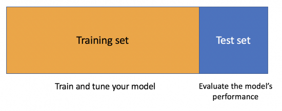
A common machine learning strategy is to take all available data and split it into training and testing subsets, usually with a ratio of 70-80 percent for training and 20-30 percent for testing. ITSI uses the training subset to train and predict patterns in the data. The train partition has a single and essential role: it provides the raw material from which the predictive model is generated. ITSI uses the test data to evaluate the performance of the trained model.
For example, if the training data predicts a health score of 60, and the test data shows a score of 62, the model has very high performance. ITSI evaluates predictive performance by comparing predictions on the test data set with actual values using a variety of metrics. Usually, you use the model that performed best on the test subset (the "recommended" model) to make predictions on future health scores.
By default, ITSI selects a random 70 percent of the source data for training and uses the other 30 percent for testing. Use the slider in the training section to specify a custom split ratio.
Consider the following guidelines when splitting your data:
- Always split your data before training a model. This is the best way to get reliable estimates of a model's performance.
- After splitting your data, don't change the test period until you choose your final model. The test period is meant for retraining purposes.
- When dealing with large data sets (for example, 1 million data points), a larger split of 90:10 is a good choice.
- With a smaller data set (for example, 10,000 data points), a normal split of 70:30 is sufficient.
- In most cases, the more training data you have, the better the result will be.
| Determine whether your service is a good fit for modeling in ITSI | Test a predictive model in ITSI |
This documentation applies to the following versions of Splunk® IT Service Intelligence: 4.11.0, 4.11.1, 4.11.2, 4.11.3, 4.11.4, 4.11.5, 4.11.6, 4.12.0 Cloud only, 4.12.1 Cloud only, 4.12.2 Cloud only, 4.13.0, 4.13.1, 4.13.2, 4.13.3, 4.14.0 Cloud only, 4.14.1 Cloud only, 4.14.2 Cloud only, 4.15.0, 4.15.1, 4.15.2, 4.15.3, 4.16.0 Cloud only, 4.17.0, 4.17.1, 4.18.0, 4.18.1, 4.19.0, 4.19.1, 4.19.2, 4.19.3, 4.19.4, 4.20.0, 4.20.1


 Download manual
Feedback submitted, thanks!