Understanding the fit and apply commands

The Splunk Machine Learning Toolkit (MLTK) uses the fit and apply search commands to train and fit a machine learning model, sometimes referred to as a learned model.

At the highest level:

• The fit command produces a learned model based on the behavior of a set of events.
• The fit command then applies that model to the current set of search results in the search pipeline.
• The apply command repeats the field selection of the fit command steps.

This document explains how the fit and apply commands train and apply the machine learning model based on an algorithm. These commands modify the events from the sample data you input into Splunk. All the sample data ingested serves as examples for the machine learning model to train on.

Before training the model, data may need to be cleaned up in order to remove gaps in data, clean up data or remove erroneous data.

This document walks through the fit and apply commands with example data. In this example, we want to predict field_A from all the other fields in the data available.

What the fit command does

The Machine Learning Toolkit performs these steps when the fit command is run:

1. Search results are pulled into memory.
2. The fit command transforms the search results in memory through these data preparation actions:
   1. Discard fields that are null throughout all the events.
   2. Discard non-numeric fields with more than (>) 100 distinct values.
   3. Discard events with any null fields.
   4. Convert non-numeric fields into "dummy variables" by using one-hot encoding.
   5. Convert the prepared data into a numeric matrix representation and run the specified machine learning algorithm to create a model.
3. Apply the model to the prepared data and produce new (predicted) columns.
4. Learned model is encoded and saved as a knowledge object.

Search results are pulled into memory

When you run a search, the fit command pulls the search results into memory, and parses them into Pandas DataFrame format. The originally ingested data is not changed.

Discard fields that are null throughout all the events

In the search results copy, the fit command discards fields that contain no values.

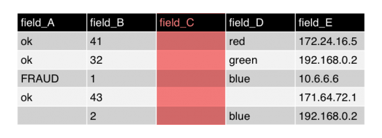
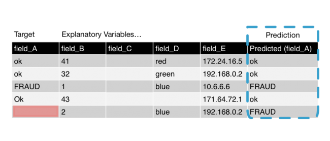
The following example demonstrates how the fit command looks for incidents of fraud within a dataset. It shows a simplified visual representation of the search results. As part of data preparation, field_C is highlighted to be removed because there are no values in this field.

If you do not want null fields to be removed from the search results, you must change your search. For example, to replace the null values with 0 in the results for field_C, you can use the SPL fillnull command. You must specify the fillnull command before the fit command, as shown in the following search example:

... | fillnull field_C | fit LogisticRegression field_A from field_*

Discard non-numeric fields with more than (>) 100 distinct values

In the search results copy, the fit command discards non-numeric fields if the fields have more than 100 distinct values. In machine learning many algorithms do not perform well with high-cardinality fields, because every unique, non-numeric entry in a field becomes an independent feature. A high-cardinality field leads to an explosion in feature space very quickly.

In the fit command example, none of the fields have a non-numeric field with more than 100 distinct values, so no action is taken.

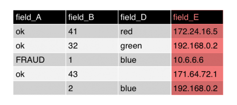
Should the search results have had more than 100 distinct Internet Protocol (IP) addresses in field_E it would qualify as high-cardinality. The IP numbers get interpreted as non-numeric or string values. The fit command would remove field_E from the search results copy in that case.

One alternative is to use the values in a high-cardinality field to generate a usable feature set. For example, by using SPL commands such as streamstats or eventstats, you can calculate the number of times an IP address occurs in your search results. You must generate these calculations in your search before the fit command. The high-cardinality field is removed by the fit command, but the field that contains the generated calculations remains.

The limit for distinct values is set to 100 by default. You can change the limit by changing the max_distinct_cat_values attribute in your local copy of the mlspl.conf file. See Configure the fit and apply commands for details on updating the mlspl.conf file attributes.

Prerequisites

• Only users with file system access, such as system administrators, can make changes to the mlspl.conf file.
• Review the steps in How to edit a configuration file in the Admin Manual.

Never change or copy the configuration files in the default directory. The files in the default directory must remain intact and in their original location. Make the changes in the local directory.

Steps

1. Open the local mlspl.conf file. For example, $SPLUNK_HOME/etc/apps/Splunk_ML_Toolkit/local/.
2. Under the [default] stanza, specify a different value for the max_distinct_cat_values setting.

Discard events with any null fields

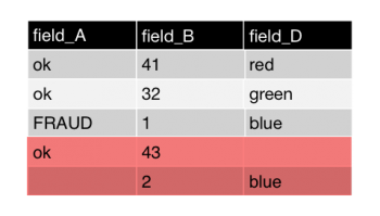
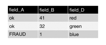
To train a model, the machine learning algorithm requires all of the search results in memory to have a value. Any null value means the entire event will not be contributed to the learned model. The fit command example dropped every column that is entirely null, and now it drops every row (event) that has one or more nulls.

Alternatively, you can specify that any search results with null values be included in the learned model. Choose to replace null values if you want the algorithm to learn from an example with a null value, and to return an empty collection. Or choose to replace null values if you want the algorithm to learn from an example with a null value, and to throw an exception.

To include the results with null values in the model, you must replace the null values before using the fit command in your search. You can replace null values by using SPL commands such as fillnull, filldown, or eval.

Convert non-numeric fields into "dummy variables" by using one-hot encoding

In the search results copy, the fit command converts fields that contain strings or characters into numbers. Algorithms expect numerically scored data, not strings or characters. The fit command converts non-numeric fields to binary indicator variables (1 or 0) using one-hot encoding.

When the fit command converts non-numeric fields using one-hot encoding, strings, characters, and other non-numeric values for each field are encoded as binary values (1 or 0). In this example field_D, which previously contained strings and characters, is converted to three fields: field_D=red, field_D=green, field_D=blue. The values for these new fields are either 1 or 0. The value of 1 is placed in the search results where the color name appeared previously. For example, in the new field field_D=red, a 1 appears in the first result, and zeros appear in the other results.

The following example shows the results of one-hot encoding. This change occurs internally, within the search results copy in memory.

If you want more than 100 values per field, you can use one-hot encoding with SPL commands before using the fit command.

Example:

In the following example, SPL is used to code search results without limiting values to 100 values per field:

| eval {field_D}=1 | fillnull 0

Convert the prepared data into a numeric matrix representation and run the specified machine learning algorithm to create a model

The fit command has prepared the search results copy for the algorithm. This dense numeric matrix is used to train the machine learning model. A temporary model is created in memory.

Apply the model to the prepared data and produce new (predicted) columns

The fit command applies the model to the now prepared data. These are the results that are returned from the search before the fit command is run. The model is applied to each search result to predict values for the search results, including the search results with null values.

The fit command appends one or more fields (columns) to the results. The appended search results are then returned to the search pipeline.

The following image shows the original search results with the appended field. The name of the appended field starts with Predicted and includes the name of the <field_to_predict>, as specified with the fit command. In this example, the <field_to_predict> is field_A. The name of the appended field is Predicted (field_A). This field contains predicted values for all of the results. Although there is an empty field in our target column, a predicted result still generated. This works because the predicted value is generated from all the other available fields, not from the target field value.

Learned model is encoded and saved as a knowledge object

If the algorithm supports saved models, and the into clause is included in the fit command, the learned model is saved as a knowledge object.

When the temporary model file is saved, it becomes a permanent model file. These permanent model files are sometimes referred to as learned models or encoded lookups. The learned model is saved on disk. The model follows all of the Splunk knowledge object rules, including permissions and bundle replication.

If the algorithm does not support saved models, or the into clause is not included, the temporary model is deleted.

What the apply command does

The apply command, similar to the fit command, goes through a series of steps to prepare the data for the saved model. The apply command uses the learned model to generate predictions on the supplied data

The apply command is fast to run because the coefficients created through the fit process and the resulting model artifact are computed and saved. Think of apply like a streaming command that can be applied to data.

The Machine Learning Toolkit performs these steps when the apply command is run:

1. Load the learned model.
2. The apply command transforms the search results in memory through these data preparation actions:
   1. Discard fields that are null throughout all the events.
   2. Discard non-numeric fields with more than (>) 100 distinct values.
   3. Convert non-numeric fields into "dummy variables" by using one-hot encoding.
   4. Discard dummy variables that are not present in the learned model.
   5. Fill missing dummy variables with zeros.
   6. Convert the prepared data into a numeric matrix representation.
3. Apply the model to the prepared data and produce new (predicted) columns.

Load the learned model

The learned model specified by the search command is loaded in memory. Normal knowledge object permission parameters apply.

Examples

...| apply temp_model

...| apply user_behavior_clusters

Discard fields that are null throughout all the events

This step removes all fields that have no values for this search results set.

Discard non-numeric fields with more than (>)100 distinct values

Next, apply removes all fields that have more than 100 distinct values.

The limit for distinct values is set to 100 by default. You can change the limit by changing the max_distinct_cat_values attribute in your local copy of the mlspl.conf file. See Configure the fit and apply commands for details on updating the mlspl.conf file attributes.

Prerequisites

• Only users with file system access, such as system administrators, can make changes to the mlspl.conf file.
• Review the steps in How to edit a configuration file in the Admin Manual.

Never change or copy the configuration files in the default directory. The files in the default directory must remain intact and in their original location. Make the changes in the local directory.

Steps

1. Open the local mlspl.conf file. For example, $SPLUNK_HOME/etc/apps/Splunk_ML_Toolkit/local/.
2. Under the [default] stanza, specify a different value for the max_distinct_cat_values setting.

Convert non-numeric fields into "dummy variables" by using one-hot encoding

The apply command converts fields that contain strings or characters into numbers. Algorithms expect numerically scored data, not strings or characters. This step converts non-numeric fields to binary indicator variables using one-hot encoding.

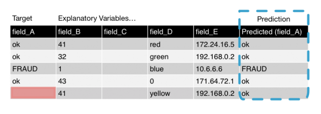
When converting categorical variables, a new value might come up in the data. In this example, there is new color data for yellow. This new data requires the one-hot encoding step, which converts column D into a binary value (1 or 0). In the graphic below, there is a new column for field_D=yellow.

Discard dummy variables that are not present in the learned model

The apply command removes data that is not part of the learned (saved) model. The data for the color yellow did not appear during the fit process. As such, the column created in the convert non-numeric fields step is discarded.

Fill missing dummy variables with zeros

Any result with missing dummy variables are automatically filled with the value 0 at this step. Doing so is a standard machine learning practice, in order for the algorithm to be applied.

Convert the prepared data into a numeric matrix representation

The apply command creates a dense numeric matrix. The model file is applied to the copy of the event and the results are calculated.

Apply the model to the prepared data and produce new (predicted) columns

The apply command returns to the prepared data and adds the results columns to the search pipeline. Although there is an empty field in our target column, a predicted result still generated. This works because the predicted value is generated from all the other available fields, not from the target field value.