Preparing your data for machine learning

Machine learning is a process of generalizing from examples. These generalizations, typically called models, are used to perform a variety of tasks, such as predicting the value of a field, forecasting future values, identifying patterns in data, and detecting anomalies from new data. Machine learning operates best when you provide a clean, numeric matrix of data as the foundation for building your machine learning models.

About the example data, SPL, and images used in this document

The examples and images in this document are based on a fictional shop and use a synthetic dataset from various source types, including web logs and point-of-sale records. This dataset does not ship with the Machine Learning Toolkit.

The sample dataset lacks the kinds of organic issues addressed in this document. As a result, you might encounter these these errors with the Search Processing Language (SPL).

1. In Compute missing values the following line of SPL drops 25% of the data, creating a scenario of missing data to compute:

   | eval method_modified = if(random() % 4 = 0, null, method)

2. In Remedy unit disagreement the following line of SPL creates unit disagreement in the response_bytes_new field by converting some data to kilobytes (by multiplying by 10 and then dividing by 1024) and some to bytes (by multiplying by 10):

   | eval response_bytes_new = if (random()%5 = 0, response_bytes * 10.0 / 1024, response_bytes * 10)

3. In Cross-validation the following line of SPL uses the eval command to manufacture valid and fraud labels into the data:

   | eval label = if (n=-81, "valid", "fraud")

If you are new to adding data and searching data in the Splunk platform, consider taking the Splunk Enterprise Search Tutorial prior to working with your data in the Machine Learning Toolkit.

Machine data preparation stages

The Splunk platform accepts any type of machine data, including event logs, weblogs, live application logs, network feeds, system metrics, change monitoring, message queues, archive files, data from indexes, and third-party data sources. Ingested data typically goes through three stages in order to be ready for machine learning.

Stage 1

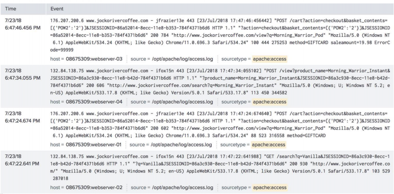
Data is ingested into the Splunk platform during the first stage. The data is typically semi-structured. You can see some commonality between the events, such as URLs and https calls in the following example:

Stage 2

After you perform some field extraction, the data is partially organized within a table. However, this table could include problems, such as missing data, non-numerical data, values in a widely-ranging scale, and words representing values. Data in the following example is not yet suitable for machine learning because the scales for the request_size and response_time are very different, which can negatively affect your chosen algorithm:

Stage 3

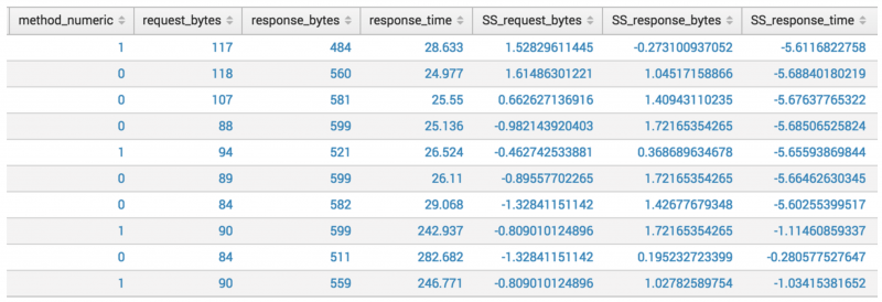
Following your completion of further field analysis and data cleaning, the data is in a clean matrix and is amenable to machine learning algorithms. This data has no missing values, is strictly numeric, and the values are scaled correctly. This data is ready for machine learning:

Identify the right data

The machine learning process starts with a question. Identify the problem you want to solve with machine learning, and use the subsequent answer as the basis to identify the data that will help you solve that problem. Ensure that the data you have is both relevant to the problem you want to solve, and that you have enough data to get meaningful results. Consider asking questions such as these:

• What data should be used to build the machine learning model?
• Do you have the right data for the type of machine learning you want to perform?
• Do you have a domain expert at your organization who you can ask about the best data to build the machine learning model?
• Is the data complete? Do you need or have access to other datasets that can support building the machine learning model?
• How should the data be weighted? Is recent data more relevant than historical data? Is data from users within an urban center more relevant that data from users in a rural area?

Data integration

If you need content from more than one dataset in order to build your machine learning model, you must integrate the datasets. When you integrate the data, use an implicit join with the OR command rather than an SQL-style explicit join.

The Splunk platform is optimized to support implicit joins. Queries using implicit joins are more efficient than those using an SQL-style join.

The following examples join user login and logout data with the session ID data. The second example uses the recommended implicit join with the OR command.

SQL-style explicit join:

sourcetype=login | join sessionID ( search sourcetype=logout)

Implicit join:

sourcetype=login OR sourcetype=logout

Clean your data

You need to clean most machine data before you can use it in machine learning. You need to clean your data in the following situations:

• The data contains errors, such as typos.
• The data has versioning issues. For example, a firmware update to a router affected how logging data is collected and how it reports on package amounts.
• The data is impacted by the upstream process, where scripts or searches add faulty fields or drop values.
• The data comes from an unreliable or out of date source that drops values.
• The data is incomplete.

Depending on the data issue, you have various methods to clean it.

Field extraction

Use field extraction techniques to integrate your data into a table. A number of fields are automatically available as a result of ingesting data into the Splunk platform, including _time and sourcetype. If the automatic field extraction options do not suffice, you can choose from technical add-ons through Splunkbase. Add-on options enable you to extract fields for certain types of data. You can also perform manual field extraction using the built-in Interactive Field Extraction (IFX) graphical workflow and iterate with regexes and delimiters to extract fields.

• To access technical add-ons, see Splunkbase.
• For more information on IFX, see Build field extractions with the field extractor.

Address missing values with fillnull command

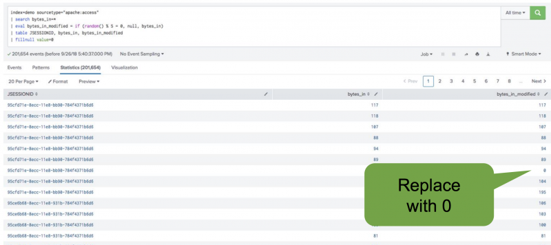
Before you can build a machine learning model, you must address missing values. The most straightforward option is to replace all the missing values with a reasonable default value, like zero. Do this by using the fillnull command.

In the following example, the fillnull command replaces empty fields with zero:

| search bytes_in=*
| table JSESSIONID, bytes_in, bytes_in_modified
| fillnull value=0

Compute missing values

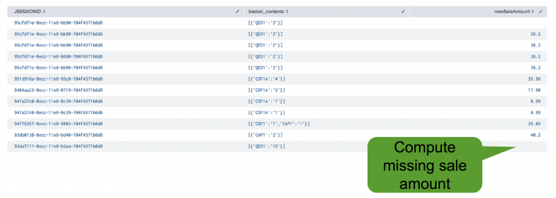
An alternative to replacing missing values with zero is to compute the missing values. For example, if your data includes the contents in an online shopping basket and you know the prices of these items, you can combine this information to calculate the missing sale amount total.

The following image shows a data set that includes values you could use to compute mssing values.

Another option uses the eval command to preserve some statistical properties of the data while replacing missing values. Using the eval command is a suitable method for scenarios in which you do not want to replace missing values with zero, but you lack a deterministic way to calculate the missing values.

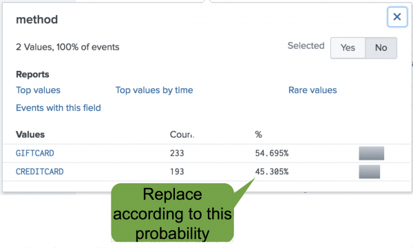
The following example uses payment method data from a website. The gift card payment method has a 54% probability of use, and the credit card has a 45% probability of use:

Use the eval command to replace missing values based on probability. The eval command acts like flipping a weighted coin, where the sides of the coin are weighted by the probability of each outcome. In this example the weights are the probability of the gift card or credit card payment method. By using this method to compute values, you preserve the distribution of the data. Missing fields are replaced according to the calculated probabilities, with 54% of the missing values replaced with gift card, and 45% of the missing values replaced with credit card.

| eval method_modified = if(random() % 4 = 0, null, method) [<- line 1 manufactures issue into data, do not copy/ paste]
| table JSESSIONID, method, method_modified
| eval method_modified_filled = if (isnull (method_modified), if (random() % 100 < 54, "_GIFTCARD", "_CREDITCARD"), method_modified)

Address missing values with the imputer algorithm

Another option to address missing values uses the imputer algorithm. The imputer algorithm replaces missing values with substitute values. Substitute values can be estimates or be based on other values in your dataset. Imputation strategies include mean, median, and most frequent. The default strategy is mean.

Pass the names of the fields to the imputer algorithm, along with arguments specifying the imputation strategy and the values representing missing data. The following example uses event information from base_action with the imputation strategy of most frequent to replace the missing values for request_bytes_new:

| eval request_bytes_new=if(random() % 3 = 0, null, base_action)
| fields - base_action
| fit Imputer request_bytes_new strategy=most_frequent
| eval imputed=if(isnull(request_bytes_new), 1, 0)
| eval request_bytes_new_imputed=round(Imputed_request_bytes_new, 1)
| fields - request_bytes_new, Imputed_request_bytes_new

After calculating the missing field, the imputer replaces the missing value with value computed by the chosen imputation strategy. To learn more about this algorithm, see Imputer algorithm.

Remedy unit disagreement

Data with very high values and very low values in a column might be the nature of the data, or it could be a case of unit disagreement. If you suspect a change occurred in the way units of data are measured, experiment with rescaling the data to see how that affects your prediction accuracy. Consider unit disagreement as a potential red-flag that's suitable for further exploration.

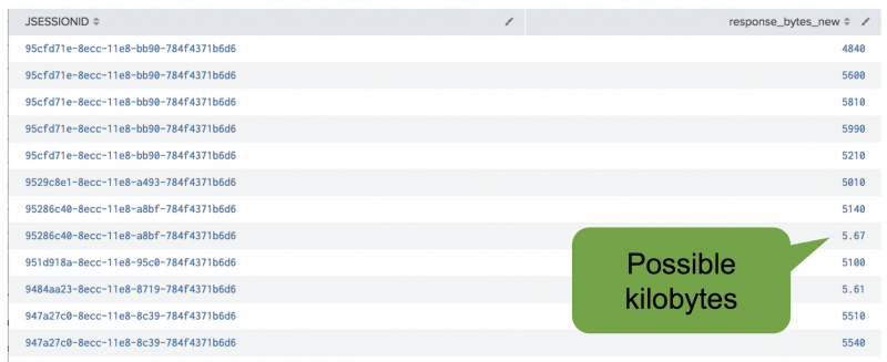
You can detect unit disagreement by using box plot charting, or by time charting the field itself, to determine if there is a change in the order of magnitude over time. The data in the following example exhibits unit disagreement in the response_bytes_new column, where some values are in the thousands and others are single digits with a decimal. In this case, the unit disagreement stems from the smaller values being measured in kilobytes rather than bytes:

When you detect unit disagreement, address the problem by converting the data to comparable units. The following example SPL shows how to convert units using test data. The second line of the search introduces a data adjustment that forces a unit disagreement issue by making some values report in kilobytes. The third line of the search rescales values that are less than 10 by multiplying those values by 1,024, the number of bytes in a kilobyte. The original column for response_bytes_new is retained in case you observe better machine learning results without rescaling.

index=demo sourcetype="apache:access" saleamount="*"
| eval response_bytes_new = if(random()%5 = 0, response_bytes * 10.0 / 1024, response_bytes * 10) [<- line 2 manufactures issue into data, do not copy/ paste]
| eval rescaled=if(response_bytes_new < 10, response_bytes_new * 1024, response_bytes_new)
| table JSESSIONID, response_bytes_new, rescaled

If you explicitly convert your data consider retaining your original data. By retaining your data, you will preserve the option to investigate and validate the hypothesis that the reporting value changed.

Address differing feature scales

Ingested data can have very different values and scales of values between columns. Value and value scale differences are normal given the nature of machine data, the different ways in which data is measured, and the amount of data available for analysis. Differing feature scales between columns does not prevent you from successfully using machine learning, but it may cause performance issues with your chosen algorithm. Look across your data for cases that might benefit from rescaling as a means to improve the accuracy of your prediction results.

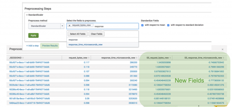
In the following example, the values in the request_bytes_new column are less than 1, whereas the values in the response_time_microseconds_new column are 100,000. You can rescale these values to improve your algorithm performance:

Rescale values between columns by using the StandardScaler algorithm. The StandardScaler algorithm is an option in the MLTK Assistants that include a Preprocessing Steps section. The specific Assistants that include built-in preprocessing are:

• Predict Numeric Fields
• Predict Categorical Fields
• Forecast Time Series
• Cluster Numeric Events

Select the fields to preprocess with respect to mean and standard deviation. When you are finished, the algorithm generates new columns of data in the data table. You can then examine the performance metrics for both the original values and the rescaled values.

Convert categorical and numeric data

Machine learning algorithms work best when you provide numeric data rather than explicit words or text. The Splunk platform can convert categorical and numeric data in different ways.

Categorical to numeric

In cases of categorical data, you can let the MLTK perform the conversion. The fit and apply commands both perform one-hot encoding on your data. After search results are pulled into memory and null events handled, fit and apply convert fields that contain strings or characters into binary indicator variables (1 or 0). This change is performed on the search results copy stored in memory.

• To learn about the specific ML-SPL commands, see ML-SPL commands.
• To learn more about the processes of the fit and apply commands, see Understanding the fit and apply commands.

Data conversion through one-hot encoding is not always the best option for your data. The following example includes data from ticketing system logs where tickets are marked as one of four categories: info, debug, warn, or critical. Converting these categorical values using one-hot encoding through the fit and apply commands results in binary numeric conversion, as seen in the following table. This manner of conversion is more useful when you want to know if values are equal or not equal.

INFO	1	0	0	0
DEBUG	0	1	0	0
WARN	0	0	1	0
CRITICAL	0	0	0	1

In cases like categorical ticket logs, the numeric conversion goes beyond telling you that the values are different, but also how the values are different. You can use the eval command to convert categorical values in combination with a case. The case operates like a switch statement, converting the example ticket categories to a corresponding number:

• If INFO, then 1.
• If DEBUG, then 2.
• If WARN, then 3.
• If CRITICAL, then 4.

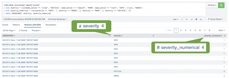
| eval severity_numerical = case(severity == "INFO", 1, severity == "DEBUG", 2, severity == "WARN", 3, severity == "CRITICAL", 4)
| table JSESSIONID, severity, severity_numerical

The output preserves the original severity column and creates a new column for severity_numerical. The severity_numerical column shows the numeric value for the corresponding ticket category:

Numeric to categorical

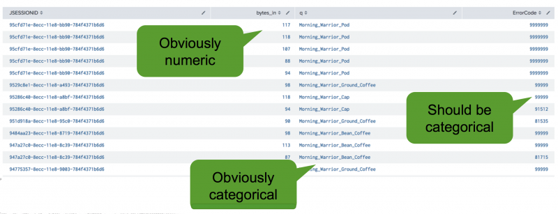
You might have data where a field is numeric, but the information from those numbers is not especially valuable. In the following example, the data includes several error code values, such as 91512, 81535, and 81715. Although the error code numbers 81535 and 81715 are closer numerically than 91512, there are no insights into what the numbers mean. You can gather more insight knowing if these values are equal or not equal by converting these numeric fields into categorical fields.

To coerce theErrorCode column from numeric to categorical, use the eval command to add a string suffix. In this example, the suffix of _str is used.

| eval ErrorCodeCategorical = ErrorCode."_str"
| table JSESSIONID, ErrorCode, ErrorCodeCategorical

The new suffix results in the content being treated as categorical. Use the fields sidebar to identify fields with a pound sign ( # ) as numeric and a cursive letter "a" as categorical.

Apply feature engineering

Features are informative values and are fields in your data that you want to analyze using machine learning. Feature engineering is the process of gleaning informative, relevant values from your data so that you can create features to train your machine learning model. Feature engineering can make your data more predictive for your machine learning outcomes and goes beyond performing data cleaning.

To successfully perform feature engineering, you must have domain knowledge.

Aggregates

Aggregates let you combine data in different ways to create more valuable data for your model training. For example, rather than clustering user data based on initial events that correspond to a single page visit, you can use aggregates to compute data by days active or visits per day to represent the users. Alternatively, rather than clustering data based on visits, you can use aggregates to produce a user type, such as power user or new user, based on data in lookup files.

The following example uses lookup files for the computed aggregates of user_activity, user_id, days_active, and visits_per_day. The fit command finds clusters based on the quantities from these lookup files:

| stats count by action user_id
| xyseries user_id action count
| fillnull
| lookup user_activity user_id OUTPUT days_active visits_per_day
| fit KMeans k=10 days_active visits_per_day

Feature interactions

Another opportunity for feature engineering is feature interactions. Do you have features that might be related and do you want to explicitly capture that relationship in your data? In the Splunk platform, you can create a new feature based on the values of original features in your data.

For example, you could get insight from user role data and user industry data as independent values towards your machine learning goals. However, given that these values are related, you might get better insight from combining these values. The same is true for values capturing escalations marked by importance or urgency. You can use the plus sign character (+ ) to perform string concatenation on two values.

The following SPL shows the +on example data:

| eval categorical_factor = role + industry 

| eval numeric_factor = importance + urgency 

Non-linearity

Feature engineering is suitable for data that's not easily separated by a linear model. You can use the eval command to introduce non-linearity and manipulate the data to use a linear model.

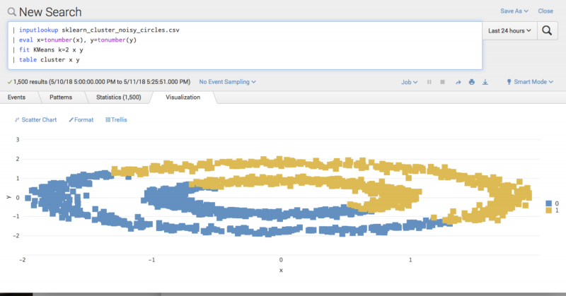
In the following visual, the example data is clustered into an inner circle and outer circle, both of which contain blue (0) and yellow (1) data points. With the current clustering, you have no way to draw a line to accurately separate these clusters. Because different algorithms work better on different data, you could consider selecting an algorithm such as DBscan to separate the clusters. A different algorithm might correct the division of clustered data, but it could also result in you losing control over the number of clusters. You can use non-linearity to compute a new field r as a function of the existing fields.

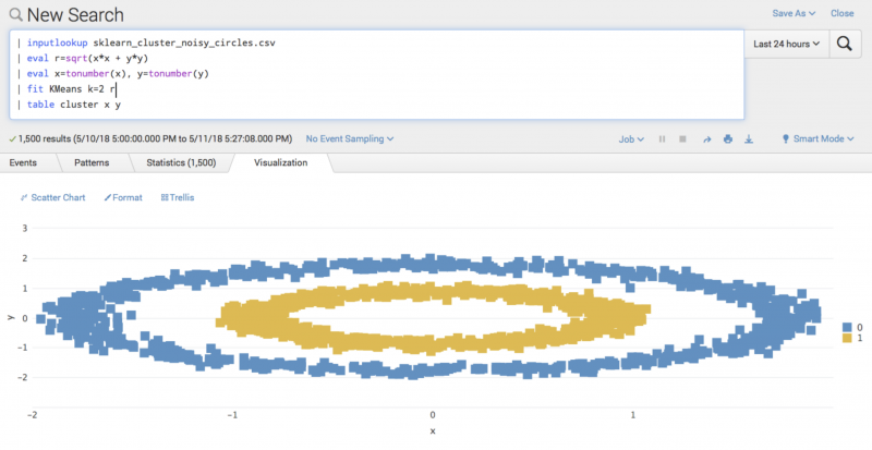
You can consider x and y as the 2 sides adjacent to the right angle of a triangle, and the new field of r as an operator of the hypotenuse of the triangle. This type of feature engineering computes the radius of the data point from a central point. When calculating r and fitting Kmeans clustering on ther field, rather than as originally calculated on x and y, feature engineering separates the 2 circles of data:

Text analytics

You can use feature engineering to perform machine learning on the basis of text data. Rather than explicitly converting text data to numeric, the term frequency-inverse document frequency (TFIDF) algorithm gives you the option to perform analytics and gain insights on text data as-is. See TFIDF algorithm.

TFIDF does not provide semantic values, such as defining which words have more meaning with respect to another metric. Semantic values are a separate metric to TFIDF. You can use lookups to bring in semantic values from another source.

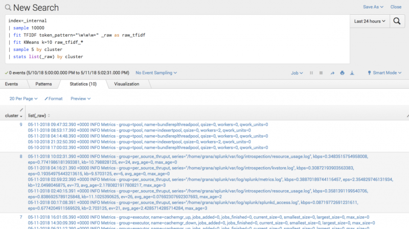
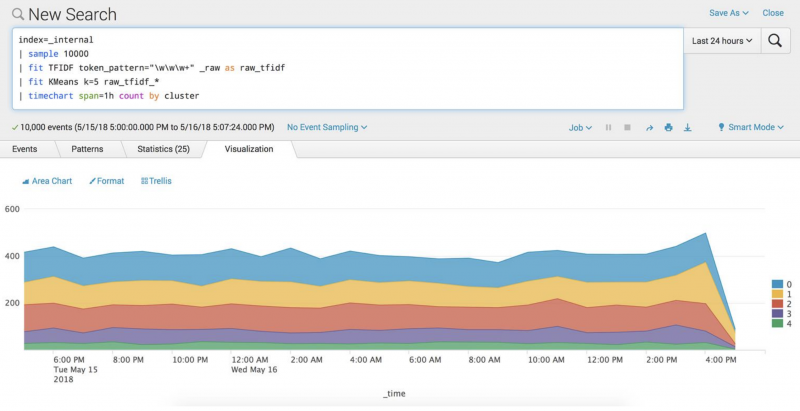
TFIDF finds words and n-grams that are common in a given event, but that are rare in your set of events. A high TFIDF score indicates that the word or n-gram is potentially important. Create TFIDF features using the TFIDF preprocessing step in the MLTK, and then use the KMeans algorithm to cluster the raw data patterns.

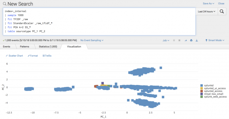
Visualizing clustered data can be informative, but you cannot visualize high-dimensional data, like the output from TFIDF. By using the PCA algorithm, you can find a low-dimensional representation of your data that also captures the most interesting variation from your original data. See PCA algorithm.

The PCA algorithm finds sets of dimensions based on your original dimensions, and can create a two-dimensional representation of your data.

You could also use a three-dimensional scatterplot add-on from to move and twist the plotted data to see the clusters more clearly. See Splunkbase.

You can choose visualization options in the MLTK to observe if clusters become more or less common over time. Data projected into a two-dimensional space with colors representing source-type clusters lets you visualize cluster changes. Add visualizations to your dashboard to see changes as they arise:

Leading indicators

Use leading indicators to increase the accuracy of your machine learning prediction or forecast. Leading indicators are sourced from data in the past, and you can use them to make future predictions based on current event data.

The following example predicts failures (FAILS) based on changes (CHANGES). Changes could stem from code commits, requested changes, or another proximal cause. You can use the streamstats command to pull information into the current event from past events. In combination with the reverse command, you can forecast future failures. By combining the streamstates and reverse commands, you can put all of your data into the same feature vector, which is a requirement for passing data to the fit command to make a prediction.

index-application_log OR index=tickets
| timechart span=1d count(failure) as FAILS count("Change Request") as CHANGES
| reverse
| streamstats window=3 sum(FAILS) current=f as FAILS_NEXT_3DAYS
| reverse
| fit LinearRegression FAILS_NEXT_3DAYS from CHANGES into FAILS_PREDICTION_MODEL

The first use of the reverse command flips time to examine future events before the past events. The streamstats command pulls data to the current event. The second use of the reverse command puts time back into the correct order, and is good practice for both SPL composition and if you need to put the results into a time-chart.

Quantization

Quantization allows you to translate multi-digit timestamps into discrete buckets. Quantized data is more readily comparable than raw timestamp data, which does not lend itself to comparison.

The following image includes timestamp data.

The following timestamp data looks like events that are far apart because the numbers are far apart. If these timestamp values were inputted into a machine learning algorithm the model would also interpret these values as being very different:

1553260380000
1552657320000
1552080679000

Quantization appropriately buckets timestamp data together. The timestamps that appeared to be different are in fact all from the same day of the week and at approximately the same time of day. Quantization allows you to group timestamp data as needed for your machine learning goals.

Friday March 22, 2019 at 1:13 pm
Friday March 15, 2019 at 1:42 pm
Friday March 8, 2019 at 1:31 pm

Data splitting

In machine learning, you don't want to train and test your model on the same data. If you test on the same data that you used to train the model, you cannot assess the quality of the generalization being produced by the model. As such, part of the process of machine learning is splitting your data so that one portion is used for training, and a separate portion is used for testing. A common data split is 70% of data for training, and 30% of data for testing.

In cases where your data lacks well-balanced examples, or you lack sufficient amounts of data, is it important to perform data splitting using more specialized methods.

Stratified sampling

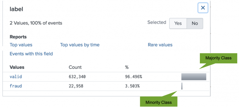
Class imbalance occurs when two classes in your data are present in different quantities. Suppose you want to use machine learning to detect instances of fraudulent transactions. Your data has limited examples of fraudulent transactions, but many examples of valid transactions. You must manage imbalanced data carefully in order to get more accurate results from your machine learning models.

The following image shows the class imbalance between the valid and fraud transaction data.

One method you can use to handle class imbalance is stratified sampling. The stratified sampling technique forces proportional representation of the minority class data.

Perform the following steps to implement stratified sampling:

1. In an example with a majority class for valid data and minority class for fraud data, begin by splitting the data into valid and fraud buckets.
2. Use the sample command to produce the partition number.
3. Include the partition number as well as a seed number in the search string. The seed number ensures that each call to the sample command produces the same partition numbers.
4. Use one call to get the training set and one call to get the test set so that each event gets the same partition number in each of the two calls. If you failed to use the same seed, you would potentially assign an event different partition numbers in each of the two calls, which could cause some events to end up in both the training and test datasets. The following SPL sets the training sets for the valid and fraud examples. A data split of 70/30 is assumed. If less than or equal to 70, the examples go into the training set.

   | search label="valid"
   | sample partitions=100 seed=1001
   | where partition_number <=70
   | outputlookup training_valid.csv
   

   | search label="fraud"
   | sample partitions=100 seed=1001
   | where partition_number <=70
   | outputlookup training_fraud.csv
   

   The following SPL shows sets up the testing set for the valid and fraud examples. A data split of 70/30 is assumed. If greater than 70, the examples go into the testing set.

   | search label="valid"
   | sample partitions=100 seed=1001
   | where partition_number >70
   | outputlookup testing_valid.csv
   

   | search label="fraud"
   | sample partitions=100 seed=1001
   | where partition_number >70
   | outputlookup testing_fraud.csv
   

   These actions result in four lookup files with 70% of the fraud examples in the training set, and the remaining 30% of the fraud examples in the testing set.
5. You can use the append command to complete building your training and testing datasets. The following example uses the append command to merge the training samples from the majority and minority classes into one training dataset.

   | inputlookup training_valid.csv | append [ inputlookup training_fraud.csv ]
   

   The following SPL example uses the append command to merge the testing samples from the majority and minority classes into one testing dataset.

   | inputlookup testing_valid.csv | append [ inputlookup testing_fraud.csv ]
   

By using stratified sampling, you can create a balanced dataset with equal representation of both your classes, giving you more power to predict the minority class of fraud.

Downsampling

Another method to address class imbalance is downsampling. Downsampling is suitable for cases with a large number of minority class examples. You can downsample the majority class to get the same number of examples.

The following image shows the disparity in classes between valid and fraud data.

Use the sample command to downsample to the smallest class. The following SPL shows the sample command on the test data.

| sample 22958 by label

Cross-validation

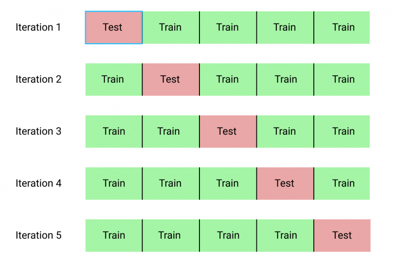
Class imbalance also occurs when you don't have large amounts of data. Cross-validation lets you use as much data as you can to train your model while allowing you to be confident that your model is generalizing well on unseen data. Cross-validation alternates holding out one piece of your data, fitting the model on the remaining data, and testing on the piece that was held out. Cross-validation repeats this pattern until all of your data is trained and tested.

Cross-validation is not well suited for time-series chart data.

Use the partition number field to leave out one partition at a time, and fit the model on the other partitions. The following SPL example shows two-fold cross-validation:

| eval label = if (n=-81, "valid", "fraud") [<- line 1 manufactures issue into data, do not copy/ paste]
| sample partitions=2 seed=43
| appendpipe [ where partition_number=0 | fit LogisticRegression label from event type date_hours state into validOrFraud ]
| where partition_number=1
| apply validOrFraud

You can also use built-in k-fold cross-validation in the MLTK. Add the kfold_cv field to the fit command to run cross-validation. To learn more about built-in k-fold cross-validation in the MLTK, see K-fold scoring.

The following diagram shows the pattern used in k-fold cross-validation of alternating holding out data for training and testing iterations:

The following SPL example shows k-fold cross-validation on a test set:

| inputlookup iris.csv 
| fit LogisticRegression species from * kfold_cv=3

Learn more

Machine data must be transformed and organized to be ready for machine learning. Tools in the Splunk platform let you identify the right data, integrate that data, clean the data, convert categorical and numeric data, apply feature engineering, and split the data for training and testing machine learning models.

Navigate to the following documents and resources to learn more about data preparation and machine learning:

• To learn how to preprocess data when using the Machine Learning Toolkit Assistants, see Preprocessing machine data using Assistants.
• To learn how to use Experiments to bring all aspects of a monitored machine learning pipeline into one interface, see the Experiments overview.
• To review the list of supported algorithms in the Machine Learning Toolkit, see Supported algorithms.
• To find a cheat sheet of ML-SPL commands and machine learning algorithms used in the Machine Learning Toolkit, download the Machine Learning Toolkit Quick Reference Guide. This document is also available in Japanese.
• To learn about implementing analytics and data science projects using Splunk's statistics, machine learning, built-in and custom visualization capabilities, see the Splunk for Analytics and Data Science course.