Maps
Use a map to visualize geospatial data on a map area of your choice. Geospatial data combines your data sets with coordinates on Earth to visually represent quantities and spread across locations.
Generate a map
- Select the Add chart button (
 ) in the editing toolbar and browse through the available charts. Choose the map.
 - Select the map on your dashboard to highlight it with the blue editing outline.
- Set up a new data source by selecting + Create search and adding a search to the SPL query window. Or, you can select an existing data source under the Search, Saved search, or Chain search sections.
- Maps with marker clusters use the SPL
tablecommand. - Maps with bubble clusters use the SPL
geostatscommand. - For example, the following are two different searches. The first is a search for marker layers and the second is a search for bubble layers.
| inputlookup geomaps_data.csv
| iplocation device_ip
| table bytes device_ip lat lon
| inputlookup geomaps_data.csv
| iplocation device_ip
| geostats latfield=lat longfield=lon count by method
- Maps with marker clusters use the SPL
- (Optional) You can also write a new ID that describes the search better than the default by changing the ID in Data source name.
- Select Apply and close.
Set a tile for the base map
Change your map's background by setting a tile for your base map with the options baseLayerTileServer and baseLayerTileServerType. Valid types for baseLayerTileServerType include "vector" and "raster". Types depend on whether the URL set for baseLayerTileServer is a vector or raster map tile.
For more details about options for maps, see Source options for maps.
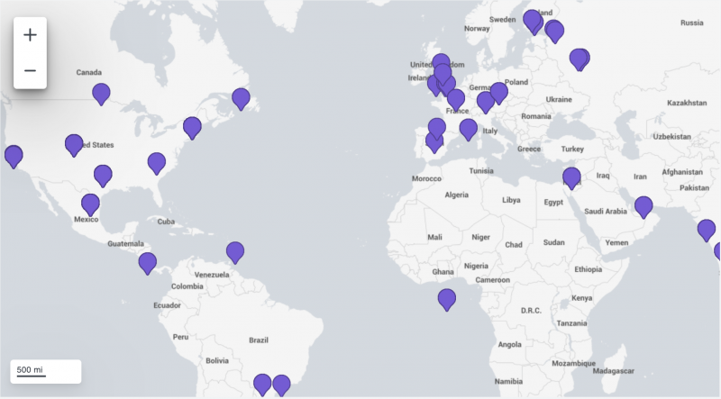
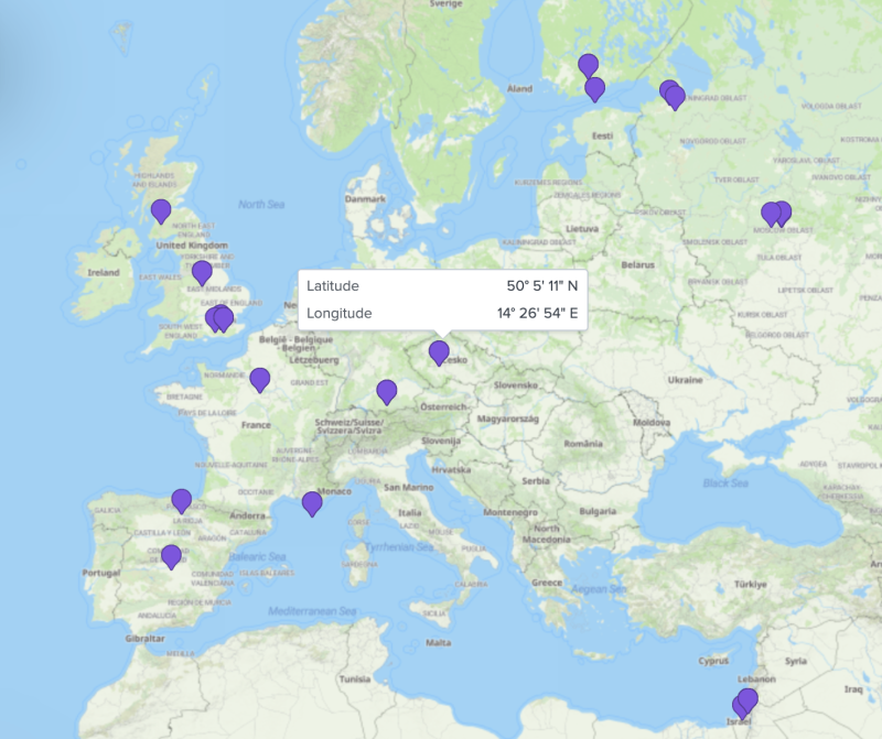
The following map visualization uses a raster tile for a base map.
Source code
Expand the window to see the source code example for setting a tile for a base map. Notice how baseLayerTileServer uses a raster map tile from a URL.
{
    "visualizations": {
        "viz_lsqZJ7UN": {
            "type": "splunk.map",
            "options": {
                "layers": [
                    {
                        "type": "marker",
                        "latitude": "> primary | seriesByName('lat')",
                        "longitude": "> primary | seriesByName('lon')"
                    }
                ],
                "center": [
                    15.121212505317928,
                    -54.48385692078051
                ],
                "zoom": 1.482683999151066,
                "baseLayerTileServer": "https://api.maptiler.com/maps/outdoor/{z}/{x}/{y}.png?key=NmOL38t5MnH6pNq8if7p",
                "baseLayerTileServerType": "raster"
            },
            "dataSources": {
                "primary": "ds_lfaIoBgK"
            },
            "context": {},
            "showProgressBar": false,
            "showLastUpdated": false
        }
    },
    "dataSources": {
        "ds_lfaIoBgK": {
            "type": "ds.search",
            "options": {
                "query": "| inputlookup geomaps_data.csv\n| iplocation device_ip\n| table bytes device_ip lat lon"
            },
            "name": "Search_1"
        }
    },
    "defaults": {
        "dataSources": {
            "ds.search": {
                "options": {
                    "queryParameters": {
                        "latest": "$global_time.latest$",
                        "earliest": "$global_time.earliest$"
                    }
                }
            }
        }
    },
    "inputs": {
        "input_global_trp": {
            "type": "input.timerange",
            "options": {
                "token": "global_time",
                "defaultValue": "-24h@h,now"
            },
            "title": "Global Time Range"
        }
    },
    "layout": {
        "type": "absolute",
        "options": {
            "width": 1440,
            "height": 960,
            "display": "auto"
        },
        "structure": [
            {
                "item": "viz_lsqZJ7UN",
                "type": "block",
                "position": {
                    "x": 0,
                    "y": 0,
                    "w": 800,
                    "h": 600
                }
            }
        ],
        "globalInputs": [
            "input_global_trp"
        ]
    },
    "description": "",
    "title": "Example of a tile server for maps"
}
Configuration panel options
You can use the Configuration panel to configure the following map components.
Title
Give your visualization a name. The title name is also helpful when searching for individual visualizations in the dashboard definitions and is not the same as the automatically assigned unique ID.
Description
Give your visualization a description to explain what the user is viewing.
Data sources
Choose an existing search or create a new one.
Visibility
Optionally hide the visualization when data is unavailable.
Position and size
You can use your mouse or the Position and size section of the Configuration panel to change the size or location of the visualization for pixel-perfect sizing and placement.
Data configurations
Select the map's layer type.
- The Marker layer type uses map pins to visualize data and clusters.
- Select the Latitude list to pick the data source for the visualization's latitude.
- Select the Longitude list to pick the data source for the visualization's longitude.
- The Bubble layer type uses differently sized circles or pie charts to visualize data and clusters.
- Select the Latitude list to pick the data source for the visualization's latitude.
- Select the Longitude list to pick the data source for the visualization's longitude.
- Select the Size list to pick the visualization's bubble size data source.
- The Choropleth layer type uses differently colored map areas to visualize distinct data concentrations.
- Select the Region Area IDs list to pick the field from your data source for the type of geographical area you want visualized with data.
- Select the Values list to pick the data source for measuring results.
Data display
Optionally select the latitude and longitude of the initial map location, and turn on or off the zoom controls.
Color and style
Select colors for the map, toggle the base layer on or off, and modify the corner radius of the visualization.
Interactions
Use drilldown to create interactivity with the different map layers. For example, with drilldown, users can click on a bubble to set a token which you can use to open a secondary search using the clicked values. For more details about setting tokens, see Setting tokens on a visualization click.
Source code
Select your visualization or its search to view and edit the source code in real-time. You can also change the Visualization ID to a more readable ID to help identify this visualization in the source code.
Marker map example
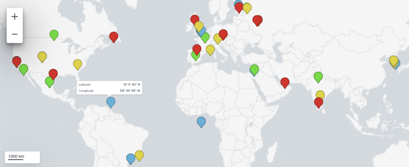
This marker map example uses config to create differently colored marker clusters to demonstrate a range of HTTP requests across geographical regions. The colors indicate varying numbers of requests based on the following ranges:
- 3001 or more requests are red
- 2001-3000 requests are blue
- 1001-2000 requests are yellow
- 1000 or fewer requests are green
Source code
The following is the source code for the marker map example.
{
    "visualizations": {
        "viz_marker_cluster": {
            "type": "splunk.map",
            "options": {
                "center": [
                    24.29483056343649,
                    2.4662060255499227
                ],
                "zoom": 1.3915833226487502,
                "layers": [
                    {
                        "type": "marker",
                        "latitude": "> primary | seriesByName(\"lat\")",
                        "longitude": "> primary | seriesByName(\"lon\")",
                        "dataColors": "> primary | seriesByName(\"bytes\") | rangeValue(config)"
                    }
                ]
            },
            "context": {
                "config": [
                    {
                        "from": 3001,
                        "value": "#de1d20"
                    },
                    {
                        "from": 2001,
                        "to": 3000,
                        "value": "#54afda"
                    },
                    {
                        "from": 1001,
                        "to": 2000,
                        "value": "#ded41d"
                    },
                    {
                        "to": 1000,
                        "value": "#4ade1d"
                    }
                ]
            },
            "dataSources": {
                "primary": "ds_x7YkfW2Y"
            }
        }
    },
    "dataSources": {
        "ds_x7YkfW2Y": {
            "type": "ds.search",
            "options": {
                "query": "| inputlookup geomaps_data.csv\n| iplocation device_ip\n| table bytes device_ip lat lon"
            },
            "name": "Search_1"
        },
        "ds_TMfPIhsl": {
            "type": "ds.search",
            "options": {
                "query": "| inputlookup geomaps_data.csv\n| iplocation device_ip\n| table bytes device_ip lat lon"
            },
            "name": "Search_2"
        },
        "ds_4QzeZfAB": {
            "type": "ds.search",
            "options": {
                "query": "| inputlookup geomaps_data.csv\n| iplocation device_ip\n| geostats latfield=lat longfield=lon count"
            },
            "name": "Search_3"
        },
        "ds_DHERK2tc": {
            "type": "ds.search",
            "options": {
                "query": "| inputlookup geomaps_data.csv\n| iplocation device_ip\n| geostats latfield=lat longfield=lon count by method"
            },
            "name": "Search_4"
        }
    },
    "defaults": {
        "dataSources": {
            "ds.search": {
                "options": {
                    "queryParameters": {
                        "latest": "$global_time.latest$",
                        "earliest": "$global_time.earliest$"
                    }
                }
            }
        }
    },
    "inputs": {
        "input_global_trp": {
            "type": "input.timerange",
            "options": {
                "token": "global_time",
                "defaultValue": "-24h@h,now"
            },
            "title": "Global Time Range"
        }
    },
    "layout": {
        "type": "absolute",
        "options": {
            "display": "auto-scale"
        },
        "structure": [
            {
                "item": "viz_marker_cluster",
                "type": "block",
                "position": {
                    "x": 30,
                    "y": 30,
                    "w": 1010,
                    "h": 420
                }
            }
        ],
        "globalInputs": [
            "input_global_trp"
        ]
    },
    "description": "",
    "title": "Marker Cluster Map example"
}
Bubble map example
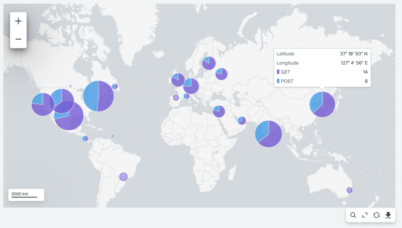
The following bubble map example uses bubble clusters to demonstrate the type and number of HTTP requests in different geographic regions.
Source code
The following is the source code for the bubble map example.
{
   "visualizations": {
       "viz_bubble_cluster": {
           "type": "splunk.map",
           "options": {
                "layers": [
		    {
		        "type": "bubble"
		    }
		]
           },
           "dataSources": {
               "primary": "ds_DHERK2tc"
           }
       }
   },
   "dataSources": {
       "ds_x7YkfW2Y": {
           "type": "ds.search",
           "options": {
               "query": "| inputlookup geomaps_data.csv\n| iplocation device_ip\n| table bytes device_ip lat lon"
           },
           "name": "Search_1"
       },
       "ds_TMfPIhsl": {
           "type": "ds.search",
           "options": {
               "query": "| inputlookup geomaps_data.csv\n| iplocation device_ip\n| table bytes device_ip lat lon"
           },
           "name": "Search_2"
       },
       "ds_4QzeZfAB": {
           "type": "ds.search",
           "options": {
               "query": "| inputlookup geomaps_data.csv\n| iplocation device_ip\n| geostats latfield=lat longfield=lon count"
           },
           "name": "Search_3"
       },
       "ds_DHERK2tc": {
           "type": "ds.search",
           "options": {
               "query": "| inputlookup geomaps_data.csv\n| iplocation device_ip\n| geostats latfield=lat longfield=lon count by method"
           },
           "name": "Search_4"
       }
   },
   "defaults": {
       "dataSources": {
           "ds.search": {
               "options": {
                   "queryParameters": {
                       "latest": "$global_time.latest$",
                       "earliest": "$global_time.earliest$"
                   }
               }
           }
       }
   },
   "inputs": {
       "input_global_trp": {
           "type": "input.timerange",
           "options": {
               "token": "global_time",
               "defaultValue": "-24h@h,now"
           },
           "title": "Global Time Range"
       }
   },
   "layout": {
       "type": "absolute",
       "options": {
           "display": "auto-scale"
       },
       "structure": [
           {
               "item": "viz_bubble_cluster",
               "type": "block",
               "position": {
                   "x": 20,
                   "y": 20,
                   "w": 940,
                   "h": 490
               }
           }
       ],
       "globalInputs": [
           "input_global_trp"
       ]
   },
   "description": "",
   "title": "Bubble cluster example"
}
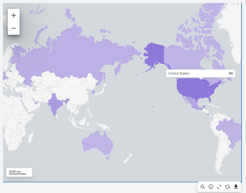
Choropleth map example
The following map uses IP address location to demonstrate the geographical areas with the highest concentration of unique IP addresses.
Source code
The following is the source code for the choropleth map example.
{
  "visualizations": {
    "viz_epnyq5z8": {
      "type": "splunk.map",
      "options": {
        "center": [
          5.684341886080802e-14,
          -122.41949999999997
        ],
        "zoom": 0.22881867003789005,
        "layers": [
          {
            "type": "choropleth",
            "areaIds": "> primary | seriesByName('country')",
            "areaValues": "> primary | seriesByName('count')"
          }
        ]
      },
      "dataSources": {
        "primary": "ds_YyFf4bor"
      }
    }
  },
  "dataSources": {
    "ds_YyFf4bor": {
      "type": "ds.search",
      "options": {
        "query": "| inputlookup geomaps_data.csv\n| iplocation device_ip\n| lookup geo_countries latitude AS lat longitude AS lon OUTPUT featureId AS country\n| stats distinct_count(device_ip) by country\n| geom geo_countries featureIdField=country"
      },
      "name": "Search_1"
    }
  },
  "defaults": {
    "dataSources": {
      "ds.search": {
        "options": {
          "queryParameters": {
            "latest": "$global_time.latest$",
            "earliest": "$global_time.earliest$"
          }
        }
      }
    }
  },
  "inputs": {
    "input_global_trp": {
      "type": "input.timerange",
      "options": {
        "token": "global_time",
        "defaultValue": "-24h@h,now"
      },
      "title": "Global Time Range"
    }
  },
  "layout": {
    "type": "absolute",
    "options": {
      "width": 1440,
      "height": 960,
      "display": "auto"
    },
    "structure": [
      {
        "item": "viz_epnyq5z8",
        "type": "block",
        "position": {
          "x": 0,
          "y": 0,
          "w": 800,
          "h": 600
        }
      }
    ],
    "globalInputs": [
      "input_global_trp"
    ]
  },
  "description": "",
  "title": "Choropleth layer example"
}
Source options for maps
The following options are available for editing maps in the source editor.
| Property | Type | Default | Description |
|---|---|---|---|
| backgroundColor | string | > themes.defaultBackgroundColor | Specify the color for the background. You can use a data source or hexadecimal code to apply the color. |
| center | number | n/a | Specify the map's center using latitude and longitude. The center might automatically set or result in [0,0] coordinates depending on available data. |
| layers | object[] | [object Object],[object Object] | Specify the data visualization layers on top of the base map. The layer can also be empty and only show the base map. |
| scaleUnit | ("metric" | "imperial") | metric | Specify which scale unit to use. |
| showScale | boolean | TRUE | Specify whether to show the scale on the bottom left. |
| baseLayerTileServer | string | n/a | Specify the tile set URL for the base map. For example, you might use street tiles for a neighborhood map or terrain tiles for a mountain range map. |
| baseLayerTileServerType | ("vector" | "raster") | n/a | Specify the type of tile set for the base map. Valid types include "vector" and "raster". |
| zoom | number | n/a | Specify the zoom level of the map. |
layers (object type)
The following are nested options that you can set in the layers section of the visualization stanza.
| Property | Type | Default | Description |
|---|---|---|---|
| type | ("marker" | "bubble") | bubble | Specify the type of data layer method to display points on the map. For example, "bubble" or "marker". |
| bubbleSize | (string | array) | frameBySeriesTypes("number") | Specify the data column to encode bubble size. This applies to layers where the type is "bubble". |
| latitude | (string | array) | > primary | seriesByName("latitude") | Specify a data source to apply latitude coordinates for data points displayed on the map. |
| longitude | (string | array) | > primary | seriesByName("longitude") | Specify a data source to apply longitude coordinates for data points displayed on the map. |
| dataColors | (string | array) | n/a | Specify the colors used for data points. If specified, this option overrides the seriesColors option. You can use a data source or an array of colors to apply the coloring. For example, " > primary | seriesByName("status") | matchValue(colorMatchConfig)". |
| seriesColors | string[] | ["#7B56DB", "#009CEB", "#00CDAF", "#DD9900", "#FF677B", "#CB2196", "#813193", "#0051B5", "#008C80", "#99B100", "#FFA476", "#FF6ACE", "#AE8CFF", "#00689D", "#00490A", "#465D00", "#9D6300", "#F6540B", "#FF969E", "#E47BFE"] | Specify the colors used for data points. If the dataColors option is specified, the seriesColors option is ignored. |
| additionalTooltipFields | string[ ] | [ ] | Specify the fields to add to the default set of tooltips. Tooltips appear when you hover over data points. These fields and their corresponding values will be shown in addition to those displayed by default. |
| resultLimit | number | 1000 | Specify the maximum number of data points to render on the map. |
| Link graphs | Parallel coordinates |
This documentation applies to the following versions of Splunk Cloud Platform™: 9.1.2308, 9.1.2312, 9.2.2403, 9.0.2305
 Download manual
Feedback submitted, thanks!