About the fit and apply commands
The fit and apply commands are 2 of the custom machine learning (ML) Splunk Search Processing Language (SPL) commands included in the Splunk Machine Learning Toolkit (MLTK). These ML-SPL commands implement classic machine learning and statistical learning tasks.
The fit command trains and saves a model from search results. The apply command applies that model to new search results to provide predictions or other insights.
The fit and apply commands work on relative searches with relative time ranges, but will not complete on real-time searches.
Before you begin
Before training your own models, your data might benefit from preprocessing. Data preprocessing can help address missing values, remedy unit disagreements, convert categorical data to numeric, and more. Running the fit command does include some lightweight data preprocessing, but a clean, numeric matrix of data is best for building your machine learning models.
To learn about data preprocessing options see Preparing your data for machine learning and Preprocessing your data using the Splunk Machine Learning Toolkit.
Actions taken by the fit command
The following actions take place when the fit command is run:
The fit command modifies a model. The command is considered risky because running it can cause performance issues. As a result, this command triggers SPL safeguards. To learn more, see
Search commands for machine learning safeguards.
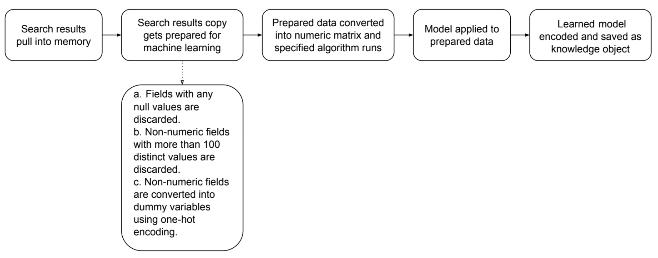
Search results pull into memory
When you run the fit command the search results pull into memory, a copy is created of the search results, and the search results are parsed into a Pandas DataFrame format.
The originally ingested data is not changed.
Search results copy gets prepared for machine learning
Your data must be prepared to make it suitable for machine learning. The following actions all take place on the search results copy.
| Action | Description |
|---|---|
| Fields with any null values are discarded | The fit command discards fields that contain no values. To train a model, the machine learning algorithm requires all search results have a value. Any null value means the entire event will not contribute towards the learned model. The fit command discards any fields that are null throughout all of the events, and drops every event that has one or more null fields.
If you do not want null fields to be removed from the search results you must change your search. You can specify that any search results with null values be included in the learned model. Or choose to replace null values if you want the algorithm to learn from an example with a null value and to return an empty collection. Or choose to replace null values if you want the algorithm to learn from an example with a null value and to throw an exception. To include the results with null values in the model, you must replace the null values before using the |
| Non-numeric fields with more than 100 distinct values are discarded | The fit command discards non-numeric fields if the fields have more than 100 distinct values. In machine learning, many algorithms do not perform well with high-cardinality fields, because every unique, non-numeric entry in a field becomes an independent feature.
The limit for distinct values is set to 100 by default. You can change the limit by changing the Only users with admin permissions can make changes to the mlspl.conf file. To learn more about changing .conf files, see How to edit a configuration file in the Splunk Admin Manual. An alternative to discarding fields is to use the values to generate a usable feature set by using SPL commands such as To learn more about data preprocessing options see Preparing your data for machine learning. |
| Non-numeric fields are converted into dummy variables using one-hot encoding | Algorithms perform best with numeric data rather than categorical data. The fit command converts fields that contain strings or characters into numbers. The fit command makes this conversion using one-hot encoding. One-hot encoding converts categorical values to the binary values of 1 or 0.
|
Prepared data converted into numeric matrix and specified algorithm runs
The prepared data is converted into a numeric matrix that's ready to be processed by the selected algorithm, and trained to become the machine learning model. A temporary model is created in memory.
Model applied to the prepared data
The fit command applies the temporary model to the prepared data. The fit command appends one or more columns to display the results. The appended search results are then returned to the search pipeline.
Learned model encoded and saved as knowledge object
When the temporary model file is saved, it becomes a permanent model file. These permanent model files are sometimes referred to as learned models or encoded lookups. The learned model is saved on disk. The model follows all of the Splunk knowledge object rules, including permissions and bundle replication.
When the chosen algorithm supports saved models, and the into clause is included in the fit command, and the learned model is saved as a knowledge object. If the algorithm does not support saved models, or the into clause is not included, the temporary model is deleted.
Actions taken by the apply command
The apply command completes several actions to re-convert data learned when running the fit command. The apply command generally runs on a small slice of data that is different data than that used for training the model with the fit command. The apply command generates insights into new columns.
Coefficients created through the fit command and the resulting model artifact are already computed and saved, making the apply command fast to run. The apply command operates like a streaming command applied to data.
The following actions take place when the apply command is run:

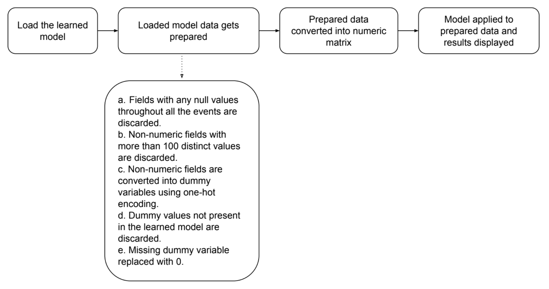
Load the learned model
The learned model specified by the search command is loaded in memory. Standard knowledge object permissions are used. The following are examples of the apply command loading the learned model:
...| apply temp_model
...| apply user_behavior_clusters
Loaded model data gets prepared
The data must be properly prepared to be suitable for machine learning and running though the selected algorithm. The following actions all take place on the search results copy.
| Action | Description |
|---|---|
| Fields with any null values throughout all the events are discarded | The apply command discards fields that contain no values.
|
| Non-numeric fields with more than 100 distinct values are discarded | The apply command discards non-numeric fields if the fields have more than 100 distinct values.
The limit for distinct values is set to 100 by default. You can change the limit by changing the Only users with admin permissions can make changes to the mlspl.conf file. To learn more about changing .conf files, see How to edit a configuration file in the Splunk Admin Manual. |
| Non-numeric fields are converted into dummy variables using one-hot encoding | Algorithms perform better with numeric data, versus categorical data. The apply command converts fields that contain strings or characters into numbers using one-hot encoding. The apply command converts non-numeric fields to the binary variables of 1 or 0.
|
| Dummy values not present in the learned model are discarded | The apply command removes data that is not part of the learned model.
|
| Missing dummy variable replaced with 0 | Replacing missing fields with 0 is a standard machine learning practice that's required for the algorithm to be applied. Any result with missing dummy variables are automatically filled with the value of 0. |
Prepared data converted into numeric matrix
The prepared data is converted into a numeric matrix. The model file is applied to this matrix and the results are calculated.
Model applied to prepared data and results displayed
The apply command returns to the prepared data and adds the results columns to the search pipeline.
See also
See the following resources for additional information on ML-SPL commands in MLTK:
- To learn about the other ML-SPL commands, see Search commands for machine learning.
- To follow examples of ML-SPL commands being used to train, apply, and tune a model on sample data for different scenarios including outlier detection and anomaly detection see MLTK deep dives overview.
- To learn about limiting access to ML-SPL commands, see Search commands for machine learning permissions.
- To learn about the available algorithms in MLTK, see Algorithms in the Splunk Machine Learning Toolkit.
| Search commands for machine learning permissions | Search commands for machine learning safeguards |
This documentation applies to the following versions of Splunk® Machine Learning Toolkit: 5.5.0

 Download manual
Feedback submitted, thanks!