Machine Learning Toolkit Overview in Splunk Enterprise Security

The Splunk Machine Learning Toolkit (MLTK) is replacing Extreme Search (XS) as a model generation package in Enterprise Security (ES). MLTK can scale at larger volume and also can identify more abnormal events through its models. See Welcome to the Machine Learning Toolkit in the Splunk Machine Learning Toolkit User Guide.

In an effort to improve performance and save space as compared to XS, MLTK behaves differently. As an example, XS runs on a schedule, such as daily, over a short time window. Then XS stores its models, and many of the searches merge daily data into those models, so that the historical data grows bigger over the course of a year. MLTK also runs on a schedule, such as daily, but over a bigger time window. MLTK does not merge the daily data, but replaces it with every run. The MLTK data does not grow as large and remains more relevant to the current timeframe.

Fit and apply commands

The main commands that are replacing the XS commands are fit and apply. The default correlation searches that use XS in ES are updated for you. If you have any custom correlation searches that are using XS commands, you need to revise them accordingly. See Convert Extreme Searches to Machine Learning Toolkit.

Creating models and finding anomalies

XS and MLTK are similar in many ways:

• Both XS and MLTK create models.
• Both XS and MLTK represent distributions in their models.
• Both XS and MLTK in ES use "low", "medium", "high" and "extreme" to represent threshold values. For details about threshold values, see Machine Learning Toolkit Macros in Splunk Enterprise Security.
• XS and MLTK both use their models to find outliers.
• Both use thresholds like "above high" to define what values to consider as outliers.

Creating models with xscreateddcontext versus with fit

XS uses both xscreateddcontext and xsupdateddcontext to build models. MLTK uses fit to build models.

The xscreateddcontext command creates a new model each time the context gen search is run. The following example shows a context gen search that uses xsupdateddcontext:

tstats summariesonly=true allow_old_summaries=true count as web_event_count from datamodel=Web.Web by Web.src, Web.http_method, _time span=24h | rename "Web.*" as * | where match(http_method, "^[A-Za-z]+$") | stats count(web_event_count) as count min(web_event_count) as min max(web_event_count) as max avg(web_event_count) as avg median(web_event_count) as median stdev(web_event_count) as size by http_method | eval min=0 | eval max=median*2 | xscreateddcontext name=count_by_http_method_by_src_1d container=web class="http_method" app="SA-NetworkProtection" scope=app type=domain terms="minimal,low,medium,high,extreme" | stats count

The xsupdateddcontext command merges the new results into the existing model each time the context gen search is run. The following example shows a context gen search that uses xsupdateddcontext:

tstats `summariesonly` count as failures from datamodel=Authentication.Authentication where authentication.action="failure" by authentication.src,_time span=1h | stats median(failures) as median, min(failures) as min, count as count | eval max = median*2 | xsupdateddcontext app="sa-accessprotection" name=failures_by_src_count_1h container=authentication scope=app | stats count

The fit command builds a model, replacing the data each time the model gen search is run, and the apply command lets you use that model later. The following example shows a model gen search that uses fit:

tstats `summariesonly` count as failure from datamodel=Authentication.Authentication where Authentication.action="failure" by Authentication.src,_time span=1h | fit DensityFunction failure dist=norm into app:failures_by_src_count_1h

The fit command using the DensityFunction with partial_fit=true parameter, updates the data each time the model gen search is run, and the apply command lets you use that model later. Specifying dist=norm with partial_fit will do nothing if a model already exists, so the distribution used is that of the original model. The following example shows a model gen search that uses fit and partial_fit=true :

tstats `summariesonly` count as failure from datamodel=Authentication.Authentication where Authentication.action="failure" by Authentication.src,_time span=1h | fit DensityFunction failure partial_fit=true dist=norm into app:failures_by_src_count_1h

Finding anomalies with xswhere versus apply

XS and MLTK both use their models to find outliers. Both use thresholds like "above high" to define what values to consider as outliers. For example, if you use "above high", then xswhere or apply functions show all values that are above the highest 5% (0.05). If you change this to "above extreme", then the values are above the highest 1% (0.01).

The following example shows a search that uses xswhere:

tstats `summariesonly` count as web_event_count from datamodel=web.web by web.src, web.http_method | `drop_dm_object_name("web")` | xswhere web_event_count from count_by_http_method_by_src_1d in web by http_method is above high

The following example shows a search that uses apply:

tstats `summariesonly` count as web_event_count from datamodel=Web.Web by Web.src, Web.http_method | `drop_dm_object_name("Web")` | `mltk_apply_upper("app:count_by_http_method_by_src_1d", "extreme", "web_event_count")`

To verify the qualitative IDs and thresholds, use the following search: | inputlookup qualitative_thresholds_lookup

qualitative_id	qualitative_label	threshold
extreme	extreme	0.01
high	high	0.05
medium	medium	0.1
low	low	0.25
minimal	minimal	0.5

Finding outliers with DensityFunction

Anomalies and outliers are not necessarily bad, they're just different. As you gather data over time, you'll start to recognize what's standard. You might notice deviation from past behavior or you might notice deviation from peers. As you think about the deviation, then you'll start to consider upper and lower bounds from the standard. Outside of the bounds is where you'll find your anomalies and outliers.

The DensityFunction's distribution is normal, exponential, or gaussian. ES searches are explicitly configured with the normal DensityFunction setting of dist=norm for those that use fit. You can modify the type of distribution for each MTLK model when using the fit command. Valid values for the dist parameter include: norm (normal distribution), expon (exponential distribution), gaussian_kde (Gaussian Kernel Density Estimation distribution), and auto (automatic selection). See Anomaly Detection in the Splunk Machine Learning Toolkit User Guide.

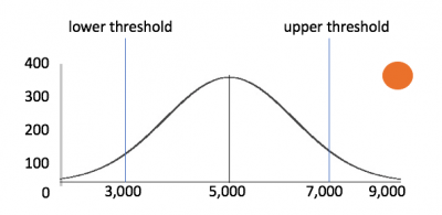
The threshold parameter is the center of the outlier detection process. It represents the percentage of the area under the density function and has a value between 0.000000001 (refers to ~0%) and 1 (refers to 100%). The threshold parameter guides the DensityFunction algorithm to mark outlier areas on the fitted distribution. For example, if threshold=0.01, then 1% of the fitted density function will be set as the outlier area.

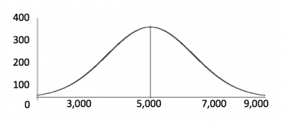
The shape of a normal distribution is that of a bell curve. Consider the scenario of network traffic volume over time. Maybe most of the traffic occurs during certain cycles. The data is naturally in a normal bell curve.

The x-axis is values. The y-axis is the number of times you see that particular value. If you see a slight increase compared to the number of times you usually see a value, it's not necessarily an outlier that you need to investigate. But if you see a large spike compared to the number of times you usually see a value, then it's probably important to investigate because it's outside the normal bounds of your upper or lower threshold.

Not all data is naturally in the shape of a bell curve, so you might need to use the "auto" dist parameter to help you find the accurate shape of your data. For example, your data might be in a Gaussian Kernel Density Estimation shape. In this case, your outliers might not be outside of upper and lower thresholds, but beyond a percentage of standard deviation.

When you're exploring your data, sometimes you already have known outliers. In some cases, you want to clean up those outliers before you train your model. For example, if you have a device on your network that is doing active or passive vulnerability scans, then you want to remove that from the results. You don't need to limit this to only known outliers. For example, if you have test servers generating data that fits in the middle of the distribution curve, this will change your curve to put more weight in the middle of the curve. This is also undesirable.

Regular search:

| tstats `summariesonly` count as total_count from datamodel=Network_Traffic.All_Traffic by _time span=30m | fit DensityFunction total_count dist=norm into app:network_traffic_count_30m

Search with outliers removed from the source:
Notice filtering out the CIDR range of the test servers by using .src!=10.11.36.0/24.

|tstats `summariesonly` count as total_count from datamodel=Network_Traffic.All_Traffic where All_Traffic.src !=10.11.36.0/24 by _time span=30m | fit DensityFunction total_count dist=norm into app:network_traffic_count_30m

You can also filter out those results when you apply the data to your model.

Most people are used to analyzing with eventstats or streamstats, gathering data just in time for analysis. The difference with MLTK is that the probability density function uses averages and standard deviations for building a model. Then you can send your data as input into the model, and then output the outliers.