Analytics reference for Splunk Observability Cloud 🔗
Splunk Observability Cloud uses the analytics language SignalFlow to power all charts and detectors. You can run calculations on observability data and visualize the output in charts using SignalFlow analytics methods. To use analytics in your charts, select Add Analytics in the Plot Editor tab.
Only SignalFlow methods are available in the chart builder view. To use SignalFlow functions, select View SignalFlow to see the SignalFlow program. For more information on writing SignalFlow programs, see the Analyze data using SignalFlow topic in the Splunk Observability Cloud Developer Guide.
Use the following list to learn more about each SignalFlow analytics method, including sample calculations.
Absolute Value 🔗
SignalFlow method: abs()
Returns the absolute value of a data point. The absolute value of a number is the number without the sign.
Ceiling 🔗
SignalFlow method: ceil()
Rounds a data point up to the largest (closest to positive infinity) floating-point value that is less than or equal to the argument and is equal to a mathematical integer.
Count 🔗
SignalFlow method: count()
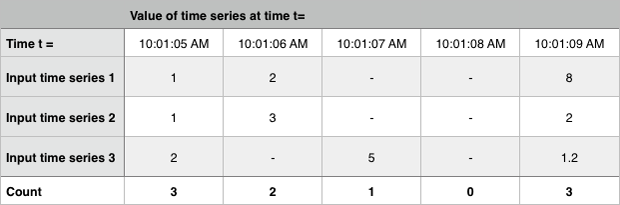
Counts the number of time series that have values, including extrapolated data points. Count is typically used to determine if data points are missing for whatever reason.
In the following example Count returns the amount of input time series which reported a data point within the time interval.
Delta 🔗
SignalFlow method: delta()
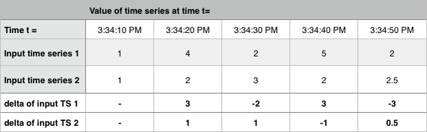
Calculates the difference between the current value and the previous value for each time interval. Delta operates independently on each time series in the plot.
In the following example, Delta returns the difference between two time series for each time interval.
EWMA and Double EWMA 🔗
SignalFlow methods: ewma() and double_ewma()
Calculates an exponentially weighted moving average (EWMA), where more recent data points are given higher weight. The weight of a data point decreases exponentially with time.
EWMA summarizes a window of data with an emphasis on points received recently. Thresholds for alerts can be set by forming a band around the EWMA using standard deviations or a percentage. Alternatively, alerting on the EWMA, much like alerting on the usual moving average, can be used in place of duration conditions.
Double EWMA, a selectable variant of EWMA, incorporates a weighted moving average of the metric’s trend, and can be used to forecast. Double EWMA addresses smoothing problems that occur when raw data exhibits a trend.
EWMA and Double EWMA parameters 🔗
Use the following parameters with EWMA and Double EWMA.
Data Smoothing (number)
Smoothing parameter, often called alpha, applied to the data points of the input time series. Must be between 0 and 1. Smaller values correspond to longer time windows and thus more smoothing (weights decay more slowly). Data Smoothing always uses the finest resolution available.
Trend Smoothing (number, applies only to Double EWMA)
Smoothing parameter, often called beta, applied to the trend of the input time series. Must be between 0 and 1. Smaller values correspond to longer time windows and thus more smoothing (weights decay more slowly). Trend Smoothin always uses the finest resolution available.
Forecast (duration, applies only to Double EWMA)
How far into the future to forecast (for example 1h, 4m, and so on). Calculated by adding an appropriate multiple of the trend term to the level term. The default value (0) smooths the series.
For example, if the forecast parameter is set to 10m, the output time series estimates the value of the input time series 10 minutes from now. This can be used to predict when a resource is likely to be exhausted, or as a way of getting alerts earlier. Forecasting also eliminates some false alarms in the scenario where the values are problematic but the trend is benign (decreasing back to healthy).
Damping (number, applies only to Double EWMA)
A number between 0 and 1. A value of 1 projects that the trend will continue indefinitely (no damping). Smaller values decay the trend towards zero as the projection gets further into the future. Damping is relevant when Forecast is not 0.
Exclude 🔗
SignalFlow methods: above() , below() , between() , not_between()
Restricts the data to be analyzed by filtering out values above or below given thresholds. You can choose whether to include the threshold values themselves. If a time series value meets the criteria set in the method, you can choose to Drop excluded points or Set excluded values to their corresponding limit.
Exclude can be useful in situations where you want to apply a condition to another analytics method. For example, if you want to count the number of servers with a CPU utilization above 80%, then you can use CPUUtilization as the metric, apply Exclude x < 80, and then apply Count.
Floor 🔗
SignalFlow method: floor()
Rounds a data point down to the smallest (closest to negative infinity) floating-point value that is greater than or equal to the argument and is equal to a mathematical integer.
Integrate 🔗
SignalFlow method: integrate()
Multiplies the values of each input time series by the resolution (in seconds) of the chart. Integrate is most useful for gauge metrics.
In the following example, Integrate calculates the change in velocity over a window of time.

For counters and cumulative counters, Integrate is less useful because a built-in Rollups with equivalent functionality already exists. For counters, applying an Integrate method to the Rate/sec (rate per second) rollup is equivalent to using the Sum rollup, assuming no missing data points. The same applies to the Delta rollup for cumulative counters.
LN or Log natural 🔗
SignalFlow method: log()
LN calculates the natural logarithm (loge) of each data point value. For each input time series, LN generates a corresponding output time series.
Log10 🔗
SignalFlow method: log10()
Calculates the common logarithm (log10) of each data point. For each input time series, Log10 generates a corresponding output time series.
Mean 🔗
SignalFlow method: mean()
Calculates the arithmetic average or mean of the available data points by dividing the sum of the values of the available data points by the number of available data points.
Types of Mean 🔗
You can choose to either aggregate or transform the values of Mean.
Mean:Aggregation
Mean across all values. Mean:Aggregation outputs an averaged time series for each group of input time series. Missing data points are treated as
nullvalues.The following example shows the averaged time series of a group of three time series.

Mean:Transformation
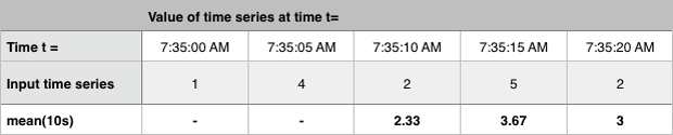
Calculates a moving average over a configurable time window. For each input time series, Mean:Transformation outputs a corresponding time series expressing for each time period the mean of the values of the input time series over a configurable time window leading up to said period. The default time window is one hour.
The following example shows a moving average calculated over a time window of 10 seconds.
The Mean method also supports transformation over a calendar window (day, week, month, and so on) and a dashboard window instead of a moving window. For more information, see Calendar window transformations and Dashboard window transformations.
Mean + Standard Deviation 🔗
SignalFlow method: mean_plus_stddev()
Applies the formula μ+n*σ, where μ is the mean, σ is the standard deviation, and n is a given number of standard deviations to add (or subtract, for negative numbers) from the mean. The default number of standard deviations is 1. The aggregation and transformation modes work in the same manner as for the independent mean and standard deviation methods.
Minimum / Maximum 🔗
SignalFlow methods: min() , max()
Returns either the smallest (Minimum) or the largest (Maximum) value seen in data points collected either from multiple time series at a point in time (aggregation), or from individual time series over a time window (transformation).
Minimum:Aggregation and Maximum:Aggregation
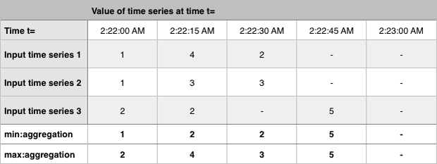
Output one time series for each group of input time series expressing, for each time period, the minimum or maximum of the values present in the input in the time period.
The following example shows the aggregated minimum and maximum for three time series.
Minimum:Transformation and Maximum:Transformation
For each input time series, outputs a corresponding time series expressing for each time period the minimum or maximum of the values of the input time series over a configurable time window leading up to that period. The default time window is one hour.
The following example shows the minimum and maximum over a time window of 10 seconds.

The Minimum and Maximum methods also support transformation over a calendar window (day, week, month, and so on) and a dashboard window instead of a moving window. For more information, see Calendar window transformations and Dashboard window transformations.
Percentile 🔗
SignalFlow method: percentile()
Finds the specified percentile of values in data points collected either from multiple time series at a point in time (aggregation), or from individual time series over a moving time window (transformation).
Percentile:Aggregation
Outputs a data stream for each group of input time series expressing, for each time period, the configured percentile (between 1 and 100, inclusive) of the values present in the input in the time period. The default percentile value is 95.
For example, by applying a percentile value of 95 to a data stream with 1,000 MTS, you get the value of the 50th biggest MTS for each time period. In this example, approximately 95% of the values are lower than the returned percentile and approximately 5% are higher.
Percentile:Transformation
For each input time series, outputs a corresponding data stream expressing, for each time period, the configured percentile (between 1 and 100, inclusive) of the input time series over a configurable time window leading up to that period. The default percentile value is 95, and the default time window is 1 hour.
For example, by requesting the 95th percentile of the past hour of an MTS with a 10s resolution (assuming no rollup), you get the 18th largest value from the past hour. In this example, out of the 360 data points from the past hour, approximately 95% of the values are lower than the returned percentile and approximately 5% are higher.
The Percentile method also supports transformation over a dashboard window instead of a moving window. For more information, see Dashboard window transformations.
Power 🔗
SignalFlow method: pow()
Raises the value of each data point to a specified power, or a specified number to the power of the data point value.
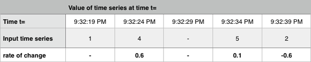
Rate of Change 🔗
SignalFlow method: rateofchange()
Calculates the difference between the current value and the previous value for each time interval, then divides the result by the length, in seconds, of that time interval.
Similar to Delta, except that it divides the difference by the time elapsed, in seconds, to normalize the change over the compute resolution.
The following example shows the rate of change over time for a time series.
Scale 🔗
SignalFlow method: scale()
Multiplies each data point by a specified number.
Scale is often used for converting values to percentages (using 100) or for converting between units of time (using 60). The default scale factor is 1.
Square Root 🔗
SignalFlow method: sqrt()
Calculates the square root of the data point values.
Standard Deviation 🔗
SignalFlow method: stddev()
The standard deviation (σ) is the square root of the variance. See Variance for how the variance is calculated for both aggregation and transformation modes.
Sum 🔗
SignalFlow method: sum()
Adds up all the values in data points collected either from multiple time series at a point in time (aggregation), or from individual time series over a time window (transformation).
Sum:Aggregation
Outputs a single time series expressing, for each period, the sum of all the values of the input time series from that same period.
Otherwise, it outputs one time series for each unique combination of the values of the grouping properties, each of those time series expressing the sum of the values of the input time series which metadata match those groups. Input time series that do not have dimensions or properties matching those grouping properties are not included in the computation and in the output.
Sum:Transformation
Calculates the sum of the values of an input time series over a moving time window. As with other transformations, an output time series is generated for each input time series. The default time window is one hour.
The following example shows both aggregation and transformation sums over a time window of 10 seconds.

The Sum method also supports transformation over a calendar window (day, week, month, and so on) and a dashboard window instead of a moving window. For more information, see Calendar window transformations and Dashboard window transformations.
Timeshift 🔗
SignalFlow method: timeshift()
Retrieves data from a previous point in time, offset by a specified time period (for example, one week), to enable comparison of a time series with its own past trends.
The presence of a Timeshift element in a plot affects the entirety of the plot it is on, regardless of its position, as it instructs SignalFlow to fetch data for all the time series of the plot with the specified time offset.
For example, a time shift of one day fetches data for time series from one day in the past, then stream the offset data in real time. This allows you to compare the current value reported in a time series with the value that was reported in the past with a constant relative offset.
The offset value can specified in weeks(w), days(d), hours(h), minutes(m), and seconds(s). The offset value is always assumed to be towards the past, and must be zero or positive. To specify an offset of two weeks and two hours, enter an offset value of 2w2h.
Note
The offset value must be greater than or equal to the minimum resolution of the data used in the current chart. For example, if you set a time shift of 30 seconds, but the resolution of your chart is five minutes, the method will be invalid.
Top and Bottom 🔗
SignalFlow methods: top() , bottom()
Can be used to select a subset of the time series in the plot.
By count
When operating by count, the output is the top or bottom N time series with the highest or lowest values in each time period, where N is the given count value. The default count value is 5.
By percent
When operating by percent, the output is the time series for which the value in each time period is higher or lower than the Pth percentile, where P is the given percentage value between 1% and 100% (inclusive). This is equivalent to the Top x% or Bottom x% of time series, by value. The default count value is 5.
A line chart using Top or Bottom shows all series that were in the Top/Bottom N at any point in the specified time window. The value for a series is replaced with null at a timestamp if that series is not in the Top/Bottom N.
Variance 🔗
SignalFlow method: variance()
The variance measures how far a set of values is spread out. Variance is calculated by dividing the sum of the squares of the difference of each value to their mean by the number of available data points.
Variance:Aggregation
Calculates the variance of values across a group of input time series at a given point in time.
Variance:Transformation
Calculates the variance of the values of an input time series over a moving time window. As with other transformations, an output time series is generated for each input time series. The default time window is one hour.